4 Infectious Disease Epidemiology
We have so far focused on epidemiology in the broadest sense, not making any difference between infectious, or communicable, and non-infectious, or non-communicable diseases. We will now begin to start looking more in detail at infectious diseases.
Infectious diseases in humans are mostly caused by biological microorganisms: viruses, bacteria, fungi, and protozoa. In addition, parasitic helminths (worms) can also cause infectious disease. Historically, infectious diseases have accompanied us ever since we came into existence. In fact, every species is confronted with infectious diseases. Even bacteria, which are the causative agents of many human infectious diseases such as the plague, cholera, or tuberculosis, are themselves getting infected by so-called phages, which are viruses that exclusively infect bacteria. Where there is life, there is infection.
For most of human history, infectious diseases have been a major killer. Only 200 years ago, countries like Germany or the UK had child mortality rates of up to 50%. A hundred years ago, every third child died before reaching age five. In 19th century Germany, only every second child would survive to that age. In Sweden during the same time period, where each woman gave birth to more than four children, every family would on average lose one child before the age of five. I mention these countries not because they were particularly affected, but simply because they began much earlier than most others to collect detailed birth and death records in their territories. We can assume that the situation was similar everywhere else in the world. Figure 4.1 shows the share of children dying before the age of five in a few countries from which we have good data.
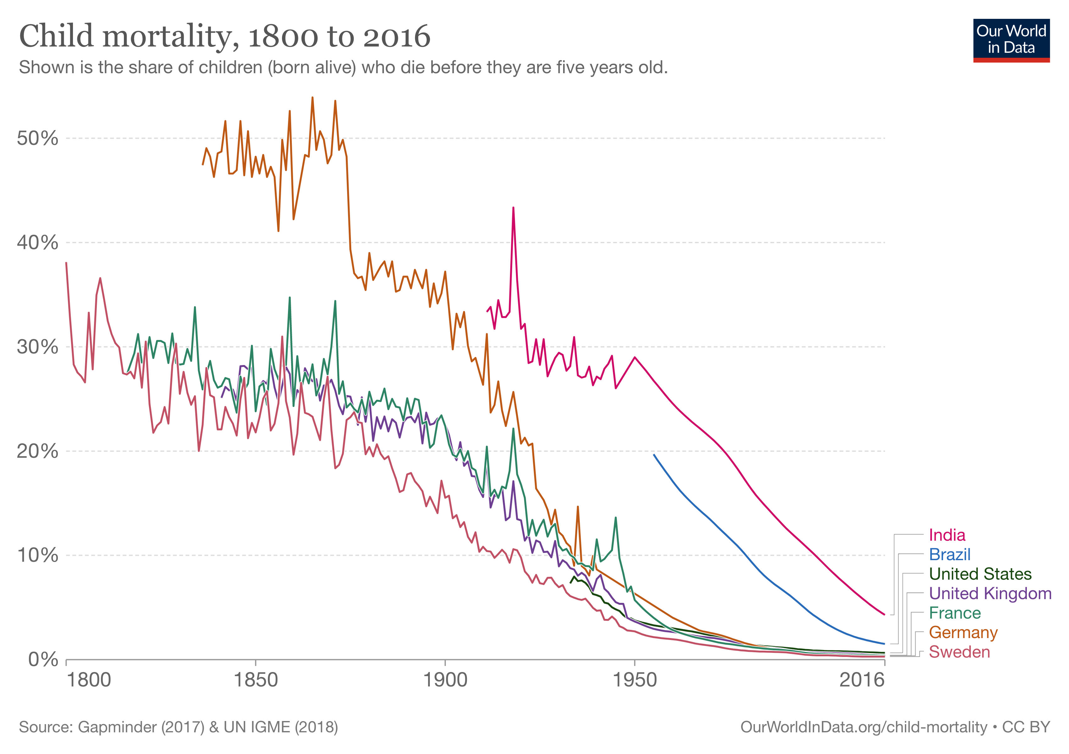
At the turn of the 19th century, these horrific numbers finally began to decline. While improvements were initially limited to Europe and the US, by the mid-20th century, child mortality rates were falling dramatically across the globe, dropping from over 30% in 1920 to under 5% in 2015. In fact, child mortality continues to fall today. In 2013, 3.6 million fewer children died than in the year 2000. This enormous progress is paralleled by the overall progress in combating infectious diseases all around the world. Thanks to better hygiene, better healthcare and social security, better prevention (for example through vaccines), and better treatments (such as antibiotics), the burden on health caused by infectious diseases has continued to fall. In many high-income countries, the mortality from infectious diseases is now just a small fraction of the mortality from non-communicable diseases. For example, in the US in the beginning of the 20th century, the two types of mortalities were roughly equal, as can be seen in Figure 4.2. But mortality due to infectious diseases, which was already on a downward trajectory then, continued to decline.
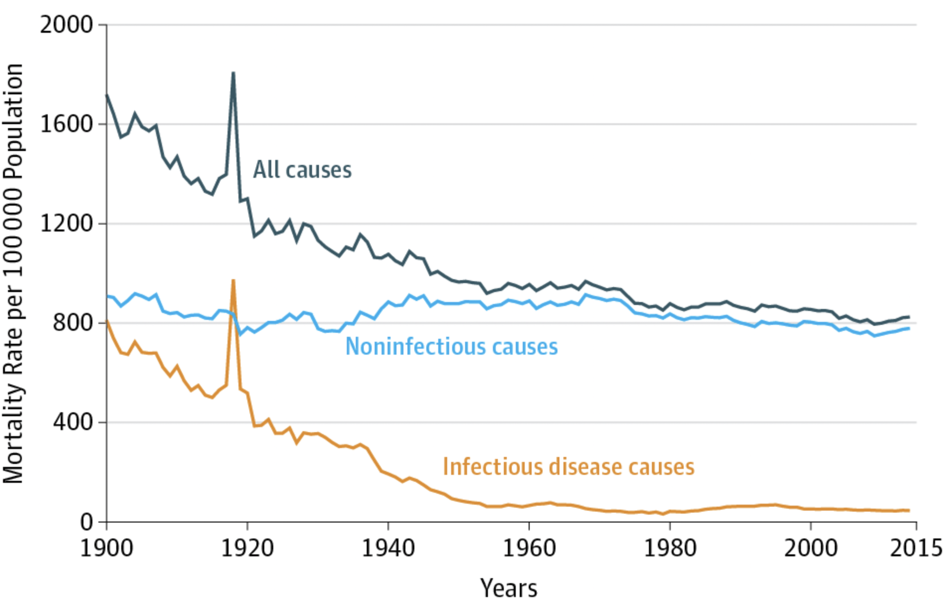
One could be tempted to look at the data and conclude that it’s not worth it anymore to invest in infectious disease prevention. But this would be wrong for numerous reasons. First, infectious diseases continue to be a leading killer in low-income countries, and they are still a substantial cause of death in middle-income countries. We understand how this mortality can be reduced, and thus have no reason not to do it. Second, we need to be careful not to reverse cause and consequence. Infectious disease mortality is low because we invest in infectious disease prevention. This is an investment that continues to yield tremendous benefits. Third, as the peak in the infectious disease mortality line before 1920 shows (Figure 4.2), the battle is never won. This peak was due to the 1918 influenza pandemic. While for many decades, the 1918 peak had to serve as the prime example of an infectious disease outbreak causing massive mortality on a global scale even in modern times, we are now - unfortunately - in a position to use a much more recent example, the COVID-19 pandemic.
For most of modern human history, medicine mistakenly believed that infectious diseases like the plague or cholera, were transmitted by foul air, or miasma. The name of the disease malaria - which literally means bad air - is a remnant of that idea, originally popularized by the Greek physicians Hippocrates and Galen. Like many mistaken medical beliefs advanced by doctors in ancient Greece, the miasma theory was accepted for over two thousand years, only to be replaced through the scientific grounding with experimental evidence of the germ theory, particularly by Louis Pasteur and Robert Koch in the second half of the 19th century. Today, we understand in great detail how infectious diseases are caused by microorganisms (and some worms), colloquially called germs; how these organisms reproduce and establish themselves in the host, thereby causing disease; and how they manage to eventually transmit themselves to individuals in a process of contagion.
In this chapter, we’ll examine the fundamentals of infectious disease epidemiology. By the end, you’ll have a strong understanding of how infectious diseases spread and how to control them. We’ll use several examples from the COVID-19 pandemic. While we can’t go back in time to prevent the pandemic, we can use this exceptional and painful event to illustrate key concepts of infectious disease epidemiology.
4.1 Emergence
Where do infectious diseases come from? As mentioned above, virtually all infectious diseases in humans are caused by viruses, bacteria, fungi, protozoa, and worms. They are among the most ancient life forms on earth (although there is still considerable debate about whether viruses should even be called alive). These organisms are parasites, which means that they live in or on their hosts, from which they extract resources. In the infectious disease context, parasitic microorganisms causing diseases are typically called pathogens. For simplicity, I will use the terms interchangeably.
Infectious diseases are likely as old as life itself. Parasitism is an inevitable consequence of evolution by natural selection, and pathogenic organisms are among the oldest life forms. The negative consequences of parasitism are serious, not only for individuals but for entire populations. For example, the fungus Batrachochytrium dendrobatidis, one of the deadliest wildlife pathogens ever documented, has driven many amphibian populations to near extinction. The Myxoma virus, which infects rabbits, has certain strains with a case fatality rate of almost 100%. Even in cases where mortality is less extreme, the selective pressure on hosts to avoid or tolerate infection can be strong enough to drive significant evolutionary adaptations. Most famously, sexual reproduction itself is thought to be driven by selection pressure imposed by parasites, an idea known as the Red Queen hypothesis. Recent human history has demonstrated the devastating effects that infectious diseases can have on local populations. Native American populations suffered dramatically from diseases such as smallpox and measles imported by Europeans, against which they had no immunity. Today, we can even study the genetic effects of severe epidemics. The devastating plague pandemic (Black Death) in the 14th century wiped out an estimated 30-50% of the European population. Those who survived had certain gene variants that conferred protection against the pathogen causing the plague (the bacterium Yersinia pestis), but are also associated with higher susceptibility to autoimmune diseases (Klunk et al. 2022).
The pathogens themselves evolve even more rapidly than their hosts. In doing so, pathogens may all of a sudden be capable of infecting species that they haven’t been capable of infecting before. For human infectious diseases, the original species from where the pathogen jumped - the reservoir species - is typically an animal species, and the disease is subsequently called zoonosis, or zoonotic disease. The reservoir species could in principle be any species, but a rather high number of zoonoses come from mammals, in particular bats and rodents (Han, Kramer, and Drake 2016). Zoonoses account for about 6 out of 10 emerging infectious diseases (K. E. Jones et al. 2008). Other sources are typically environmental, such as the soil or water. It should be noted that not all infectious diseases are novel, or emerging. Some, like chickenpox (Breuer 2020) or Hepatitis C (Ghafari et al. 2021), have coevolved with humans for thousands or tens of thousands of years, and possibly even longer.
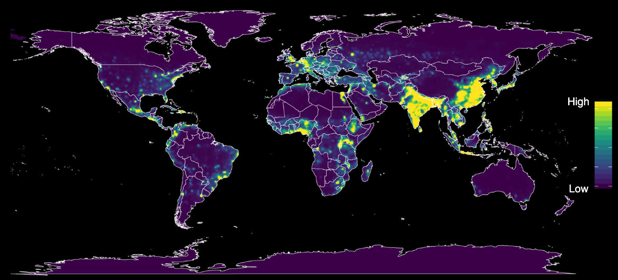
Many pathogens can infect multiple species. The jump to the human species may therefore not be particularly surprising. But for such a jump to happen, humans need to be in contact with the reservoir species. Due to the continued enlargement of human habitats through population growth and agriculture, the potential for contact between humans and reservoir species has increased substantially. This is particularly true in areas where species richness is high (Allen et al. 2017). Figure 4.3 shows a global map of predicted relative risk distribution of zoonotic events for the emergence of infectious disease, taking into account numerous human, animal, and environmental factors. Forested tropical regions show particularly high risks due to the combination of species richness and change in land use.
The event of a non-human pathogen jumping to a human host is called a spill-over event. The initial jump, however, is but the first step. The pathogen needs to be capable of establishing an infection in the new host. Because parasites have evolved mechanisms to escape their host’s immune system, the environment of a new host can pose a considerable challenge to the pathogen. Even when an infection can be established, the pathogen now needs to succeed at the final step, which is to transmit to another individual of the new host species. If this happens, the chances of a successful establishment in the new host species are very high. However, this newly initiated infection chain may still stutter and come to an end before it can take off and trigger an outbreak (Antia et al. 2003). Once a chain can establish itself, however, it can very quickly grow into an epidemic, or even a pandemic. Climate change is predicted to increase the number of spillover events further, as species can expand their geographic range, for example to higher altitudes, and new combinations of species will increase the chances of cross-species transmission (Carlson et al. 2022).
4.2 Transmission
Once a pathogen has jumped from an individual of one host species to an individual in a new host species, and managed to establish an infection, it needs to be able to transmit itself to another individual of the new species. This process of contagion is the key aspect of infectious diseases. It’s what gives infectious diseases such explosive potential, as the COVID-19 pandemic impressively demonstrated.
Transmission can occur in multiple ways. We need to differentiate between transmission modes, and transmission routes. Transmission modes describe the physical method by which pathogens are transported from one host individual to another. Transmission routes describe the physical exit and entrance location of the hosts. For example, the transmission mode of cholera is waterborne; the transmission route is generally the faecal-oral route. This means that most often, an infected person with diarrhea releases bacteria (Vibrio cholerae) into the water, and another person later drinks from the contaminated water, thereby ingesting bacteria and getting infected. We will briefly discuss the different transmission modes below.
It’s important to note that the concept of contact in infectious disease strongly depends on the mode of transmission. When talking about infectious diseases, terms like “household contacts”, “contact tracing”, “contact networks”, and others are quite common. This is because for there to be a transmission, there must be a contact in the first place. The contact is, figuratively speaking, the bridge between two hosts. A pathogen that transmits itself from one host to the next uses this bridge. But as you will see below, the nature of the bridge depends on the transmission mode.
Waterborne transmission
Waterborne transmission denotes the transmission mode by which pathogens are transmitted through water. It occurs particularly often with intestinal parasites that cause diarrhea or vomiting. Waterborne diseases include cholera, poliomyelitis (polio), and typhoid fever. The transmission route is very commonly faecal-oral. Waterborne diseases can be efficiently controlled with clean water, good sanitation infrastructure, and good hygiene. Those three aspects are often referenced by the term WASH, which is an essential part of any public health strategy. Diarrheal diseases are still one of the biggest contributors to childhood mortality2, and WASH can dramatically reduce the incidence of these diseases.
Airborne transmission: aerosol and droplet transmission
Airborne transmission denotes the transmission mode by which pathogens are transmitted through the air. Through breathing, speaking, sneezing, or coughing, an infected person produces respiratory aerosols, suspended liquid particles that contain pathogens. When those aerosols are inhaled, or otherwise deposited on the mucous membrane of another person, an infection may occur. Until recently, a difference has been made between aerosols and droplets, with the latter referring to particles larger than 5 μm that fall to the ground rapidly within 1-2 meters, while the former can remain suspended in the air. This led to the distinction between aerosol transmission, and droplet transmission. For various reasons, droplet transmission was assumed to be the dominant transmission mode for many respiratory pathogens, while aerosol transmission was generally assumed to be of minor importance. There is an interesting historical interpretation of this phenomenon, which relates to the fact that before the widespread acceptance of the germ theory of disease, miasma (foul air) was assumed to be the dominant disease transmitter, and thus any relation to airborne transmission encountered strong resistance in parts of the scientific community (Jimenez et al. 2022).
Today, thanks to investigations related to COVID-19, it is understood that aerosols up to 100 μm in size can remain suspended in the air for hours, and travel far beyond 1-2 meters (Wang et al. 2021). We further understand that the number of pathogens (or viral load when the pathogen is a virus) in aerosol is substantially higher than that of droplets. Aerosol transmission is now assumed to be an important, if not the dominant transmission mode of COVID-19, and many other respiratory diseases such as influenza. The main value of distinguishing between aerosol transmission and droplet transmission is that the latter cannot occur over long distances and extended periods of time. The previously assumed dominance of droplet transmission led to a corresponding focus on control strategies that are only partially efficient. For example, in the early stages of the COVID-19 pandemic, it was assumed that infection cannot occur beyond 1-2 meters, because droplets cannot travel beyond that distance. People were thus asked to keep their distance, and perform social distancing, or physical distancing. This was not a problem per se - even with today’s knowledge, close proximity interactions can indeed lead to many infections, not at least because aerosols are also present in close proximity. However, the erroneous focus on droplet transmission also led to the mistaken notion that transmission beyond 1-2 meters is rare or even impossible, which is clearly wrong.
The role of aerosol transmission in respiratory diseases has only recently attracted more attention. For example, influenza was commonly thought to be transmitted by droplets. Only in recent years has evidence begun to emerge that indicates that a substantial fraction of transmission is through aerosols, with far-reaching consequences (Smieszek, Lazzari, and Salathé 2019). The control of diseases transmitted through aerosols is different from the control of droplet-transmitted diseases. As aerosols are suspended in the air, ventilation and air filtration can be highly effective measures to reduce disease transmission. Facemasks are another measure to reduce airborne disease transmission, but as aerosols and droplets are differentiated by their size, different types of facemasks have different impacts on the reduction of aerosol or droplet transmission (Howard et al. 2021).
Aerosol transmission is a clear case of airborne transmission. Whether droplet transmission should also be considered part of airborne transmission, or rather a part of indirect contact transmission (fomite transmission, see below) is still a matter of debate and personal preference. Some even argue that the concept of droplet transmission should be abandoned entirely.
Contact transmission: physical contact and fomite transmission
Contact transmission denotes the transmission mode by which pathogens are transmitted through physical contact. This can occur directly, when an infected person touches another person, or indirectly via surfaces. The latter mode is called fomite transmission and occurs when an object that has previously been touched by an infected person, is touched by another person, picking up pathogens that have been deposited on the object. While the presence of pathogenic organisms on surfaces has been established beyond doubt, direct evidence for fomite transmission has been difficult to establish, not at least because it is hard to demonstrate experimentally.
Vector-borne transmission
Vector-borne transmission denotes the transmission mode by which pathogens are transmitted through a vector. A vector can be any living organism. For human infectious diseases, the most common vectors are mosquitoes and ticks, but vector species also include freshwater snails, which act as a vector for Schistosoma, parasitic flatworms that cause the disease Schistosomiasis.
Vector-borne diseases are a major killer, especially in poorer regions with a warm climate. Malaria, caused by different species of the genus Plasmodium (unicellular eukaryotes), is transmitted through mosquitoes, and caused an estimated 627,000 deaths out of 241 million cases in 20203. Other major mosquito-borne diseases are dengue fever, chikungunya fever, Zika virus fever, yellow fever, West Nile fever, and Japanese encephalitis. Climate change is expected to change the geographic range of vector-borne diseases. For example, the mosquito species Aedes aegypti, which transmits over 50 different pathogens, including the dengue virus, was originally only found on the African continent, but has now spread also to temperate regions (Kraemer et al. 2019).
Vector-borne diseases are best controlled by limiting exposure to the vector (vector control). Substantial efforts go into mosquito control, given the animal’s importance for vector-borne diseases. These efforts range from simple methods like bed nets, to historically controversial approaches like spraying DDT. In recent years, the idea of reducing the impact disease-carrying species by releasing genetically modified mosquitoes whose offspring are less likely to survive has garnered the most attention. While there is perhaps remarkable support for a human-triggered extinction event, the idea is not without controversy4.
Body fluid transmission
Infectious diseases can be transmitted through blood, semen, saliva, breastmilk, semen and vaginal secretions. This includes sexually transmitted diseases such as HIV/AIDS and Hepatitis B. However, it’s important to note that certain sexually transmitted diseases, such as syphilis and mpox, can also be transmitted through direct contact that isn’t sexual in nature. Syphilis results in sores that contain the bacteria responsible for the disease, while mpox causes lesions that have high levels of virus.
Body fluid transmission can occur during sex, childbirth, blood transfusion, and sharing of injection equipment. Which of these events can transmit a disease depends on the disease itself. For example, HIV can be transmitted through blood, semen, breast milk, and vaginal secretions, but not through saliva. On the other hand, the Epstein-Barr virus, the causative agent of mononucleosis, can easily be transmitted through saliva, even when sharing eating utensils or toothbrushes, or having contact with toys that children have drooled on.
Vertical and horizontal transmission
Vertical transmission means a disease is transmitted across generations, from parent to offspring. Horizontal transmission means that a disease can be transmitted among people that are not in a parent-offspring relationship.
Foodborne transmission
When a pathogen enters the human body through contaminated food, we speak of foodborne transmission. In contrast to many of the transmission modes mentioned above, foodborne transmission is generally part of more complex transmission chains, rather than a direct human-to-human transmission. For example, the origin of Salmonella and Norovirus - which are both among the most common foodborne pathogens - is typically an animal or water source (Stein and Chirilã 2017).
4.3 Contagion
Once a pathogen has managed to transmit within a new host species, the chances for an epidemic outbreak are very high. When one person infects another person who infects the next person, and so on, we speak of an infection chain. Early in an outbreak, infection chains can still stutter, and come to a halt. But they can also rapidly expand. Thus, in this critical phase, the dynamics of infection chains can make the difference between a very small outbreak that quickly dies out, and a pandemic.
We need a way to quantify the dynamics of contagion. This brings us to a core concept of infectious disease epidemiology: the fabled reproductive number R. R is the answer to a simple question: How many secondary cases does each case infect, on average? It’s straightforward to see that if this number is greater than 1, then the outbreak will grow, and if the number is smaller than 1, the outbreak will shrink. What is often non-intuitive is that these are typically exponential processes, at least as long as R > 1 remains roughly constant.
R0 is simply R at time point 0, i.e. at the very beginning of an outbreak. However, this time point is quite special, because it tells us something about the full potential of the pathogen, when the entire host population is still fully susceptible. This stands in contrast to Re, which is the effective reproduction number (sometimes called Rt). Re is R at any time point t > 0 during an outbreak. Re is by definition smaller than R0, because R0 assumes that everyone is susceptible except the initial case at time point 0. This is expressed mathematically as
\[R_e = R_0 * s\]
where s is the fraction of susceptibles in the population. As an outbreak progresses, and infected individuals eventually build immunity (or die), the pathogen has fewer susceptible hosts available than at the very beginning. We will look more closely at these dynamics in another chapter.
R depends on a number of factors. On the one hand, it depends on the biological properties of the pathogen itself, how well it can establish itself in the host, replicate, and its potential for transmission. However, it is a common mistake to think that R is simply a property of the pathogen. The role of the host is just as important, if not even more. The immune system is a critical determinant of a pathogen’s success in establishing, reproducing, and transmitting itself. What’s more, the host’s behavior can dramatically change R, as became very evident during the COVID-19 pandemic. For transmission to occur at all, there must be a contact in the first place. If hosts change their behaviors in such a way as to reduce the number and duration of their contacts, R will inevitably be reduced as well, and vice versa.
Estimating R during an outbreak is important, but notoriously difficult. In the ideal case, we would have a full picture of all cases, and we’d know exactly who infected whom. We would obtain this information by sequencing every infection in detail. Advances in surveillance and whole genome sequencing may one day make this possible. If we had all of this information, we would not even need to estimate R anymore - we would indeed be measuring it precisely. Until then, the most common approach is to estimate R from early outbreak data (Obadia, Haneef, and Boëlle 2012).
It’s important to note that R represents an average. If R is estimated to be 2, for example, this means that each case infects on average two new secondary cases. Understanding the distribution around this mean is important because of so-called superspreader events (Lloyd-Smith et al. 2005). A superspreader event is an event in which an index case infects many more people than R. Superspreader events are a common occurrence with SARS-CoV-2. During the COVID-19 pandemic, many superspreading events have been recorded, which have made control of the pandemic even more challenging.
The highest R values in human infectious diseases have been estimated for childhood diseases such as measles and chickenpox. Measles, for example, has an estimated R0 of about 15-20. In comparison, the R of seasonal influenza is typically around 2 or lower. The original SARS-COV-2 strain that launched the COVID pandemic was estimated to have an R0 of about 2-3. Subsequent variants have gotten more and more contagious. However, given the rapidly changing immunity landscape due to infections, re-infections, and vaccinations, estimating R0 of variants is challenging. At the time of writing, the dominant variant was the Omicron variant, which was the most contagious variant of SARS-CoV-2 so far.
4.4 Course of infection
We will now look at the course of an infection in a host. In doing so, we will encounter some key concepts along the way which will be important later on.
As we’ve seen above, the goal of any pathogen is to establish itself in a host, and transmit itself to the next host. If the host had no defenses, this entire process would be rather straightforward for the pathogen. But the host would simply be consumed in the process, which is why hosts have evolved an entire arsenal of defenses, the vast majority of which we can summarize under the term immunity. Hosts also defend themselves by physiological and anatomical barriers (e.g. the skin), and by behavioral evasion of pathogen exposure. Immune systems are among the most complex biological systems, for good reasons. They need to be able to withstand a never-ending onslaught of hundreds or thousands of different pathogens over the entire host lifetime. Any slip-up could be deadly.
All multicellular organisms have an innate immune system, which provides a very rapid (within minutes) response to infectious insults in the form of inflammation. The innate immune system is based on a limited set of receptors encoded in the germline. It includes cells such as macrophages, dendritic cells, natural killer cells, and others (Turvey and Broide 2010). It also includes humoral (i.e. in extracellular fluids) components such as antimicrobial peptides and various proteins. The innate immune system can recognize evolutionarily conserved microbial components, but has no memory, and cannot adapt over the course of a host’s lifetime. Nevertheless, given that all multicellular organisms except vertebrates rely entirely on the protection provided by the innate immune system, it would be ill-advised to dismiss the importance of innate immunity.
In addition to the innate immune system, vertebrates also have an adaptive immune system. The receptors of the adaptive immune system are adjusted based on the encounters with pathogens over a host’s lifetime, through a process of somatic recombination. The key components of the adaptive immune system are T cells and B cells (Bonilla and Oettgen 2010). T cells mature in the thymus. They have a number of important functions, such as recognizing pathogen-infected cells and killing the cell, as well as activating B cells. B cells mature in the bone marrow, and produce antibodies. They are the key actors in immune memory, which allows the immune system to remember threats it has seen before. Vaccines build on this capacity of the adaptive immune system, by training the system to learn to recognize a pathogen, without having to face the danger of a natural infection. Immune memories can be of different durations - some wane quickly, while others can last a lifetime.
When a pathogen enters the body of a person, a key question is thus whether that person has already encountered this pathogen, or a pathogen similar enough, to quickly mount a response triggered by the memory of the adaptive immune system. The innate system also provides a first line of defense. However, many pathogens have evolved sophisticated strategies to evade detection. These within-host dynamics determine the fate of the pathogen, and whether it can establish itself in sufficient numbers to eventually get transmitted to the next host. They also define the symptoms that a host will eventually experience, if any at all. Symptoms can be caused both by the pathogen itself through the damage it inflicts, and by the immune system. Fever, for example, is a response triggered by the immune system (Evans, Repasky, and Fisher 2015).
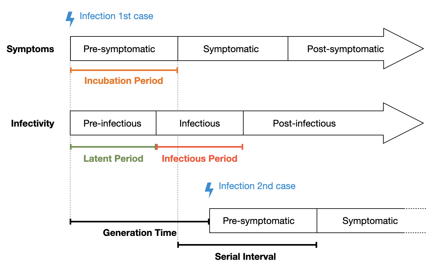
The time between initial infection and the possibility of transmission to the next host is called the latent period, or pre-infectious period. Once the latent period is over, the host enters the infectious period, which lasts until the immune system has sufficiently cleared the infection so that transmission is not possible anymore. The time between the initial infection and the appearance of symptoms is called the incubation period. Figure 4.6 shows how the incubation period and the latent period need not overlap. Indeed, these periods are of critical importance for much of disease dynamics. If the latent period is longer than the incubation period, then the host first develops symptoms before becoming infectious. This helps tremendously with control, as it is much easier to identify symptomatic patients, as opposed to asymptomatic patients. If, on the other hand, the latent period is shorter than the incubation period, a host can start to transmit the disease before being symptomatic. Indeed, such pre-symptomatic transmission is likely the key factor that made it impossible for the containment of SARS-CoV-2. This is in stark contrast to SARS-CoV-1, where people first become symptomatic before becoming infectious (Lipsitch et al. 2003), which allowed symptom-based control mechanisms (such as isolating patients) to contain the outbreak before it developed into a full pandemic. The average time it takes from the symptom onset of an index case to the symptom onset of secondary cases is called the serial interval. Note that this is similar to the average time it takes from the infection of the index case, to the infection of the secondary cases, called the generation time. However, it is generally easier to determine symptom onset than to determine the time of infection, which is why the generation time is usually estimated from the serial interval (Lehtinen, Ashcroft, and Bonhoeffer 2021).
These quantities can vary widely. For SARS-Cov-2, the mean incubation period of the Omicron variant is about 3.5 days (Liu et al. 2022), and the mean serial interval is 6.8 days (Manica et al. 2022). For influenza, the mean incubation period is about one day (Lessler et al. 2009), with a serial interval of 3-4 days (Cowling et al. 2009). For Tuberculosis, the median incubation period has been estimated to be a few months to two years (Behr, Edelstein, and Ramakrishnan 2018) - similarly for the median serial interval (Ma et al. 2018).
While the potential to infect others is limited to the infectious period, it may vary during that time, depending on factors such as viral load, and the capacity of the immune system to control the infection (T. C. Jones et al. 2021). The potential to infect others is referred to as infectivity, or infectiousness.
4.5 Heterogeneities
Once a pathogen starts to spread within a population, we’re interested in the dynamics of the spread, what factors affect it, what to expect, and what we can possibly do to control it. This is the field of infectious disease dynamics, a highly active research area where mathematical and computational models are used to simulate the processes underneath epidemics. We will look at such models in closer detail in the next chapter, where we will put to use everything we’re learning in this chapter.
What we described so far looks fairly simple: a pathogen jumps from an animal species to a human, and occasionally manages to transmit itself to other humans. We then have infection chains, which, if the conditions are met (R > 1) will lead to an outbreak. While in principle correct, this is of course a highly simplified description of what can be quite a complex process. In this section, we will look at some of the heterogeneities that are common, and known to impact the dynamics of infectious diseases. The three heterogeneities we will focus on are age, contact, and spatial heterogeneity.
Heterogeneity in age
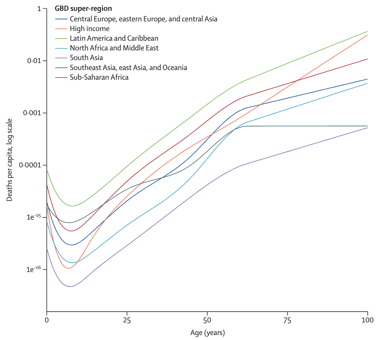
Infectious diseases do not affect all individuals equally, and age is a significant factor influencing many aspects. Age is important for a number of reasons. First, age impacts disease severity. This became strikingly obvious during the COVID-19 pandemic, where age was one of the most important predictors for disease severity, even when controlling for comorbidities (Starke et al. 2021). The age pattern of mortality (Figure 4.7) was striking, and consistent across geographies.
The cause behind this age pattern is still a matter of intense investigation. While such a pattern may seem expected, it is anything but. For example, seasonal influenza shows a similar mortality pattern, with most deaths occurring among the elderly (Iuliano et al. 2018). However, the 2009 influenza A H1N1 pandemic showed reduced mortality in the elderly, but a significant increase in excess deaths among people under 65 years (Lemaitre et al. 2012). Similarly, during the 1918/1919 influenza pandemic, mortality was greatest among the young (Simonsen et al. 1998). The dynamics of these age patterns strongly depend on the immunological history, and the subsequent immunological memory, of the population. Indeed, as we transition from a truly virgin COVID-19 epidemic that initially infected all age classes equally (though with markedly different outcomes as discussed above) to an endemic situation, it is reasonable to expect that continued reinfection will lead to increasingly mild disease in all ages, a pattern observed with other endemically circulating strains of human coronaviruses (Lavine, Bjornstad, and Antia 2021).
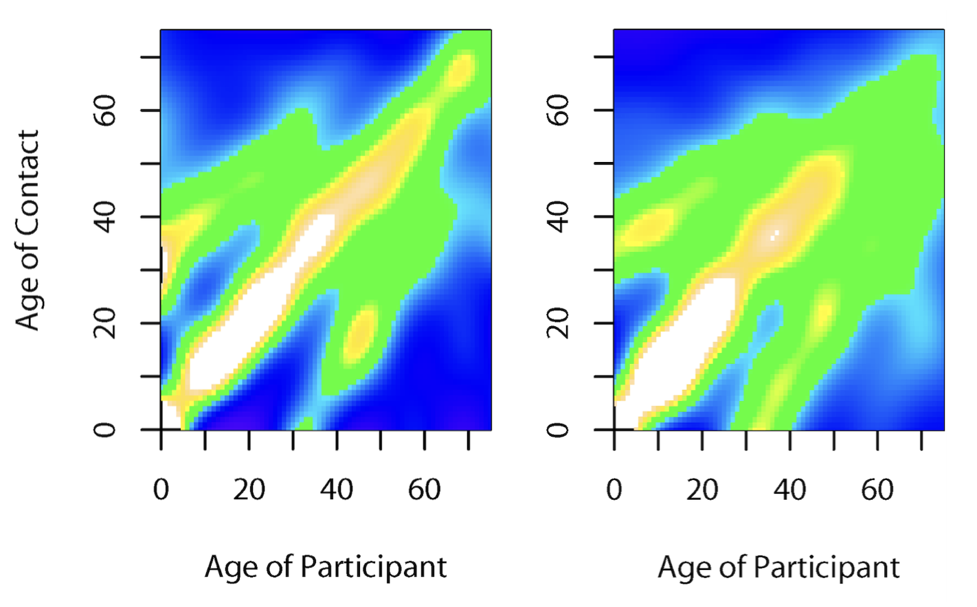
Another key factor in age is that contact patterns are highly age-stratified. While we know this intuitively and from personal experience, we also have data across different geographies (Figure 4.8), highlighting that most close-proximity contacts are in similar age groups, and across generations (parents-offspring, and teachers-students). Such assortative mixing based on age can lead to markedly different age-related prevalence patterns than those that would be expected if mixing was random (Mistry et al. 2021).
Heterogeneity in contacts
We just saw how contact patterns can strongly depend on age. Contact patterns are generally highly assortative across a number of factors. With respect to infectious disease dynamics, one of the most interesting aspects of contact heterogeneities is the number of contacts.
Contacts, as we learned earlier, depend on the transmission mode of a disease. For most contacts, if we were to make a list of all contacts of everyone in the population, we would arrive at a distribution with a certain average, and some spread around that average. Clearly, there will be people who have more contacts than others. Sexually transmitted diseases have a particularly pronounced distribution when it comes to the relevant contacts. Most people have few sexual contacts, i.e. their contacts are repeatedly with the same person. However, there are some people that have an extraordinary amount of sexual contacts, such as sex workers. It is relatively intuitive to understand that such high-contact individuals can have an outsized impact on the spread of a given infectious disease.
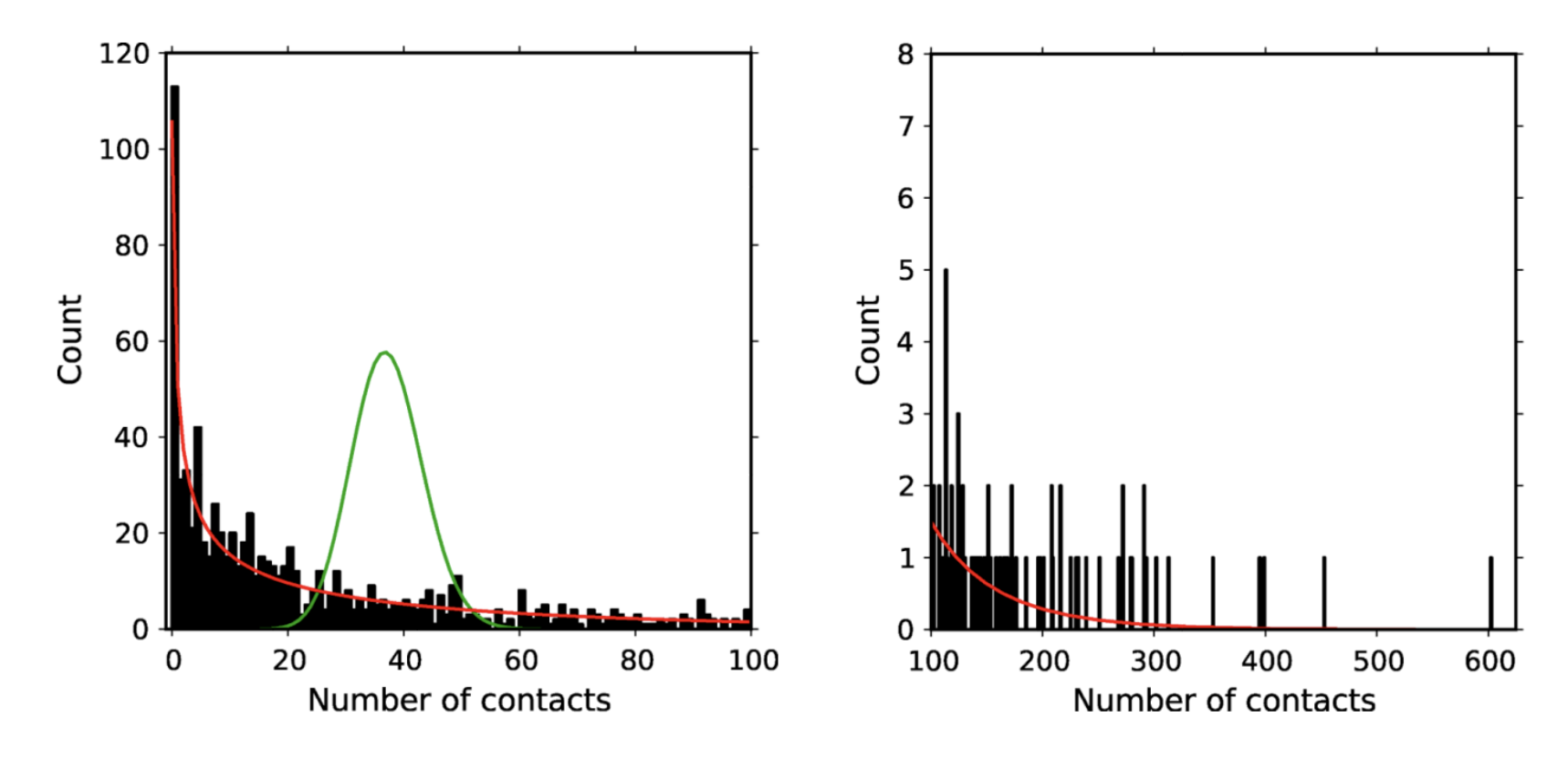
Figure 4.9 shows the number of self-reported sexual contacts from a longitudinal cohort of urban gay men observed for two years (Romero-Severson et al. 2012). As the data show, the contact distribution is highly skewed, with most men having no, or few sexual contacts, and a few men having over a hundred different sexual contacts in the same time period. The figure also shows how a simple Poisson distribution around the mean (37 contacts) in green is a very poor fit to the data, while a negative binomial distribution in red is a rather good fit, being able to capture the overdispersion in contacts.
Overdispersion in contacts has a direct effect on R0. Under the assumption of homogenous mixing, where every individual has approximately the same number of contacts, we can estimate R0 as \(r*k\), where r is the probability of disease transmission per contact, and k is the mean number of contacts. However, if there is strong overdispersion of contacts, this approximation doesn’t hold anymore. Instead, it needs to be corrected by the coefficient of variation (CV) in the contact distribution (May 2006) as follows:
\[R_0 = r*k * (1 + CV^2)\]
Thus, if the overdispersion is sufficiently strong, the resulting increase in R0 can be substantial. We will look into contact network considerations in more detail in another chapter.
Spatial heterogeneity
Hosts, such as humans, are not randomly distributed in space. Instead, they often locally cluster in subpopulations, which are connected through inter-population movement. In ecology, such a “population of populations” is called a metapopulation. Metapopulation dynamics are used in a wide range of ecological models, including those of infectious disease dynamics.
In the case of humans, the populations can be communities, villages, cities, or even countries. If within these communities, there is a high density of people, with many contacts between them, then a disease can potentially spread rapidly within these communities. Indeed, before today’s hygiene standards and widespread vaccination (at least in some parts of the world), infectious disease spread was rampant in large, high-density cities. These outbreaks would then occasionally spread to smaller communities through means of human transportation. If the density is too low, or the disease runs out of susceptible hosts, local extinction of the disease can occur. Later on, when the pool of susceptible hosts has increased sufficiently through births and immigration, a local outbreak can again occur.
A well-described example of these dynamics is found in measles. Measles is an exclusively human, highly transmissible viral disease. With an R0 estimate of up to 20, it is almost certainly the most contagious directly transmissible human pathogen (vector-borne diseases such as malaria may locally attain R0 values of 3,000 (Smith et al. 2007)). As a childhood disease, measles has in the past been responsible for millions of deaths. Because measles is so contagious, it can spread through a susceptible population very quickly. Importantly, measles is a strongly immunizing disease - meaning that infection provides lifelong sterilizing immunity - which is why it can rapidly run out of susceptibles. Unless transmission chains can be sustained through births or immigration of susceptible individuals, the disease will locally go extinct. This is where the concept of a critical community size comes in. The critical community size is the size of a community under which a disease will locally go extinct because the density of susceptible hosts is too low. For measles, the critical community size is estimated to be around 250,000 to 500,000 individuals. Above this threshold (and absent vaccines), measles can persist indefinitely, as there are always sufficient numbers of susceptible newborns to infect, and sustain transmission chains. Below this threshold, new outbreaks need to be seeded by import from other communities. Recent molecular evidence suggests that the measles virus diverged from the (now extinct) cattle pathogen Rinderpest morbillivirus about 2,600 years ago (Düx et al. 2020), a date which is in line with the rise of human urbanization and large-scale settlements.
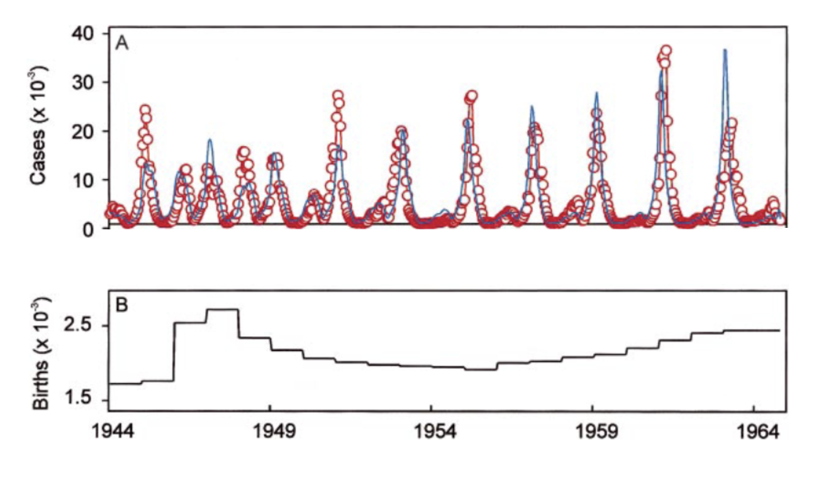
Such spatiotemporal dynamics are generally described as forest fire dynamics. Using a dataset of measles cases in the pre-vaccine era in England and Wales, measles dynamics were shown (Grenfell, Bjørnstad, and Kappey 2001) to follow a pattern of regular outbreaks in large cities, which “sparked” outbreaks in smaller towns nearby where local extinction prevented measles to persist.
Spatial dynamics thus depend critically on the transportation flows between different locations, both over shorter and longer distances. Especially the long-distance transportation flows have in recent decades expanded massively in the wake of globalization. Given the enormous international traffic flows enabled through air travel, communities on opposite sides of the planet are now just a few days away from each other. The COVID-19 pandemic once again provides a striking example of these dynamics. An outbreak that began in Wuhan, China, quickly sparked local outbreaks across the globe, which developed into a large-scale, ongoing pandemic. After first being reported in Wuhan on the 31st of December, 2019, the disease had already spread to at least 26 additional countries within one month. Digital data sources such as mobile phones provide a unique opportunity to quantify human movement, something we will look into in detail in later chapters. For example, mobile phone data provided information on the population flow through Wuhan in the early weeks of the COVID-19 pandemic, accurately predicting the frequency and geographical distribution of cases (Jia et al. 2020).
4.6 Vaccination
Vaccines are arguably one of the greatest inventions of all time. In terms of numbers of lives saved, or numbers of deaths prevented, vaccines are a strong contender for the first place, along with nitrogen-fixation technology (Haber-Bosch), blood transfusion, and other inventions that profoundly changed the course of humanity.
The concept of vaccines is deceptively simple with just a basic understanding of immunology. Vaccines essentially trick the body into developing immune memory against a pathogen, without exposing the body to the risk of a natural infection by that pathogen. A precursor to vaccination was variolation, which specifically refers to the practice of deliberate inoculation with smallpox from another patient in hope of a milder disease course (mortality ~ 2%), compared to natural infection (mortality ~30%). Variolation dates back to the 16th century or even earlier, but was later replaced by the first vaccine, the smallpox vaccine, invented by Edward Jenner. Notably, Jenner almost died of a smallpox infection caused by variolation in his childhood. Towards the end of the 18th century, Jenner built on the observation that people infected with cowpox by cattle generally did not get smallpox. Today, we understand the reasons why: cowpox infection triggers immune memory that can recognize and neutralize a smallpox infection. The early smallpox vaccine contained cowpox virus, but the active ingredient was eventually changed to vaccinia virus, which belongs to the same virus family (Poxviridae) as smallpox and cowpox. The smallpox vaccine alone saved hundreds of millions of lives, and eventually led to the only successful eradication of a human pathogen so far; but the impact on other diseases was equally profound.
The effect of vaccination depends on the type of immunity that the vaccine induces. In the same way that immunity through natural infection can be lifelong, or waning, immunity through vaccination can have various consequences. For example, vaccination with two doses of the measles vaccine provides lifelong immunity in the vast majority of people, and milder disease in those who nevertheless catch measles. In contrast, the COVID-19 vaccines famously do not provide infection-blocking immunity, but they do provide strong protection against severe disease outcomes.
There are different types of vaccines. The first type is whole pathogen vaccines, which contain whole pathogens that have either been weakened (attenuated) or killed. An example is the MMR vaccine, which contains live measles, mumps, and rubella viruses that have been attenuated. Flu vaccines also contain whole pathogens that have been weakened or killed. The second type is subunit, or acellular vaccines, which do not contain whole pathogens, but parts of it, typically parts of the surface of the pathogen, or toxoids, which are inactivated toxins that that pathogen would produce normally. The whooping cough (pertussis) vaccine is a good example, as it is composed of viral proteins and a modified version of the pertussis toxin. Notably, the pertussis vaccine is also available as a whole pathogen vaccine.
Most current vaccines are either whole pathogen vaccines or subunit vaccines. In recent decades, however, two new types of vaccines have been developed. Nucleic acid vaccines are vaccines that contain genetic instructions of the pathogen, which the machinery in human cells then uses to create pathogenic subunits (e.g. proteins). Famously, three COVID-19 vaccines are based on this technology. The vaccines by Moderna and BioNTech-Pfizer are mRNA vaccines that do not contain any viral proteins, but rather mRNA of the SARS-CoV-2 spike protein, which is then used by the human cells to manufacture the protein, triggering an immune response against it. The vaccine made by AstraZeneca uses a modified chimpanzee adenovirus - which is itself harmless for humans - as a delivery vehicle for the genetic sequence of the SARS-CoV-2 spike protein.
Vaccines, like any other pharmacological intervention, are not perfect. Their effectiveness must be continuously evaluated. Even highly effective vaccines can lead to non-intuitive phenomena. We have seen in the chapter on diagnostic tests that a highly accurate test can nevertheless have a low predictive value, if prevalence is low. A similar phenomenon occurs with highly effective vaccines under low prevalence circumstances. Consider the example of a 2014/2015 measles outbreak in California, where it was observed that over 80% of the cases were doubly vaccinated. How is this possible with a vaccine that has a 99% efficacy? We can once again turn to Bayes’ theorem, and calculate the probability of being vaccinated, given that one has been infected, \(P(V|I)\), like so:
\(P(V|I) = \frac{P(I|V) P(V)}{P(I)}\)
Let’s first look at the numerator. The probability of being infected despite vaccination, \(P(I|V)\), is \(1 - vaccine\ efficacy\), or \(1 - V_e\). The probability of being vaccinated is simply the vaccine coverage, \(c\). The numerator is thus \(c(1 - V_e)\).
The denominator, \(P(I)\), is the probability of infection, independent of vaccination status, which can come about in two ways. Either, one gets vaccinated, and then infected despite vaccination, which is \(P(V) P(I|V)\); or one doesn’t get vaccinated, and then infected without the vaccine, which is \(P(¬V) P(I|¬V)\). Thus, the full denominator is \(P(V) P(I|V) + P(¬V) P(I|¬V)\). We simplify this by replacing \(P(I|V)\) with \(1 - V_e\); \(P(V)\) by \(c\); \(P(¬V)\) by \(1-c\); and \(P(I|¬V)\) by 1, as we can safely assume that measles infection is guaranteed when not vaccinated. The denominator thus becomes \(c(1 - V_e) + 1 - c\), which further simplifies to \(1 - (c * V_e)\).
We thus have the relatively simple formula \(P(V|I) = \frac{c(1 - V_e)}{1 - (c * V_e)}\).
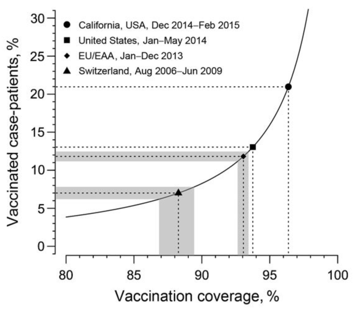
If we assume that vaccination coverage is 95%, and vaccine efficacy is 99%, we obtain a value of \(P(V|I) = 16\%\). We would thus have to expect that about 16% of those infected are vaccinated - despite the very high efficacy of the vaccine. The relationship for a number of measles outbreaks is shown in Figure 4.11.
Shortly after the rollout of the COVID-19 vaccines, similar calculations were performed when it was observed that a substantial number of vaccinated people became infected. However, as it soon became clear, the COVID-19 vaccines, unlike the measles vaccine, were not infection-blocking.
Herd immunity
As we have seen, vaccines can have two main effects. The first effect is to reduce disease severity. However, vaccines can also be infection-blocking. This is even better, because no infection automatically means no disease. With infection-blocking vaccines, we can observe the phenomenon of herd immunity, which means the additional protective effect of vaccines on those who have no immunity, either because they cannot establish it biologically, or because they are not vaccinated. Infection-blocking immunity does not only protect the immune person from getting infected and developing disease, but it also protects other people indirectly from getting infected by that person.
Disease outbreaks ultimately come to an end when the disease runs out of susceptible hosts. If an infected host cannot at least infect one other host on average (Re < 1), the outbreak will recede (and no new outbreaks will occur). Infection-blocking vaccines reduce the number of susceptible hosts, thereby reducing Re. The question thus naturally arises, what is the necessary vaccination coverage for herd immunity to be sufficiently high so that Re < 1? The answer is that under the assumption of homogenous mixing, and a random distribution of the vaccine, the necessary vaccination coverage needs to be
\[c > 1 - (\frac{1}{R_0})\]
Consider again, for example, the case of measles, assuming an R0 of 20, which means that each infection on average causes 20 more infections. It is easy to see that in order for Re to be less than 1, at least 19 - or 95% - of the 20 infections need to be prevented. It’s important to note, however, that herd immunity is not a binary outcome. The effect of herd immunity - indirect protection through fewer infected hosts - exists even when immunity is low. Colloquially, however, the term herd immunity is generally used to describe the situation when it is strong enough to stop or prevent outbreaks.
4.7 Control
Given the substantial health burden imposed by infectious diseases, there is great interest in ways to prevent, or control infectious disease spread. There is a general distinction between non-pharmaceutical interventions, or NPIs, and pharmaceutical interventions such as vaccines and antibiotics.
For pharmaceutical interventions, we can draw a further distinction between pre-exposure interventions, i.e. interventions to prevent infection, and post-exposure interventions, i.e. interventions to treat the disease (or at least to reduce or to prevent its transmission). Some post-exposure interventions, if given very early after exposure (often within hours), can prevent the development of the disease in the first place, for example in Rabies (which otherwise has a 100% lethality). For pre-exposure prevention, vaccines are the dominant pharmaceutical intervention. However, as discussed above, not all vaccines are infection-blocking, but rather reduce severity, and / or reduce the chance of transmission (Tan et al. 2023). For HIV/AIDS, where currently no vaccine exists, so-called pre-exposure prophylaxis (PrEP) in the form of antiviral drugs has been shown to be able to reduce the risk of an HIV infection with an effectiveness of close to 100% 5.
On the treatment side, the biggest impact has been made with antibiotics against bacterial infections, a revolution in medicine that has saved hundreds of millions of lives. In just about 100 years, bacterial infections have gone from being an enormous and ever-present health burden with substantial mortality, to a generally treatable condition. Before the industrial production of antibiotics, bacterial diseases such as the plague or tuberculosis would regularly kill millions of people, often in short periods of time. Simple throat or ear infections could quickly turn deadly. Antibiotics changed all of this. However, today, bacteria have evolved resistance against antibiotics. Antibiotic resistance is a serious and growing concern, with many public health agencies placing it among the top major public health concerns that need urgent addressing.
For viruses, most treatments are in the form of antiviral drugs, such as antiretroviral therapy, or ART, against HIV. Antiviral drugs against respiratory viral diseases are still rare. Oseltamivir is an antiviral drug against the influenza virus, and has been stockpiled by many governments to prepare for an eventual influenza pandemic (Colizza et al. 2007), but concerns about limited efficacy remain (Jefferson et al. 2014). For COVID-19, multiple antiviral drugs such as remdesivir and nirmatrelvir have been shown to be effective in reducing disease severity under certain circumstances (Arbel et al. 2022). Another line of treatment is provided by monoclonal antibodies (mABs), which have also been used during the COVID-19 pandemic, with mixed results (Hirsch et al. 2022). As with bacteria, there is concern about the evolution of resistance against these antiviral drugs.
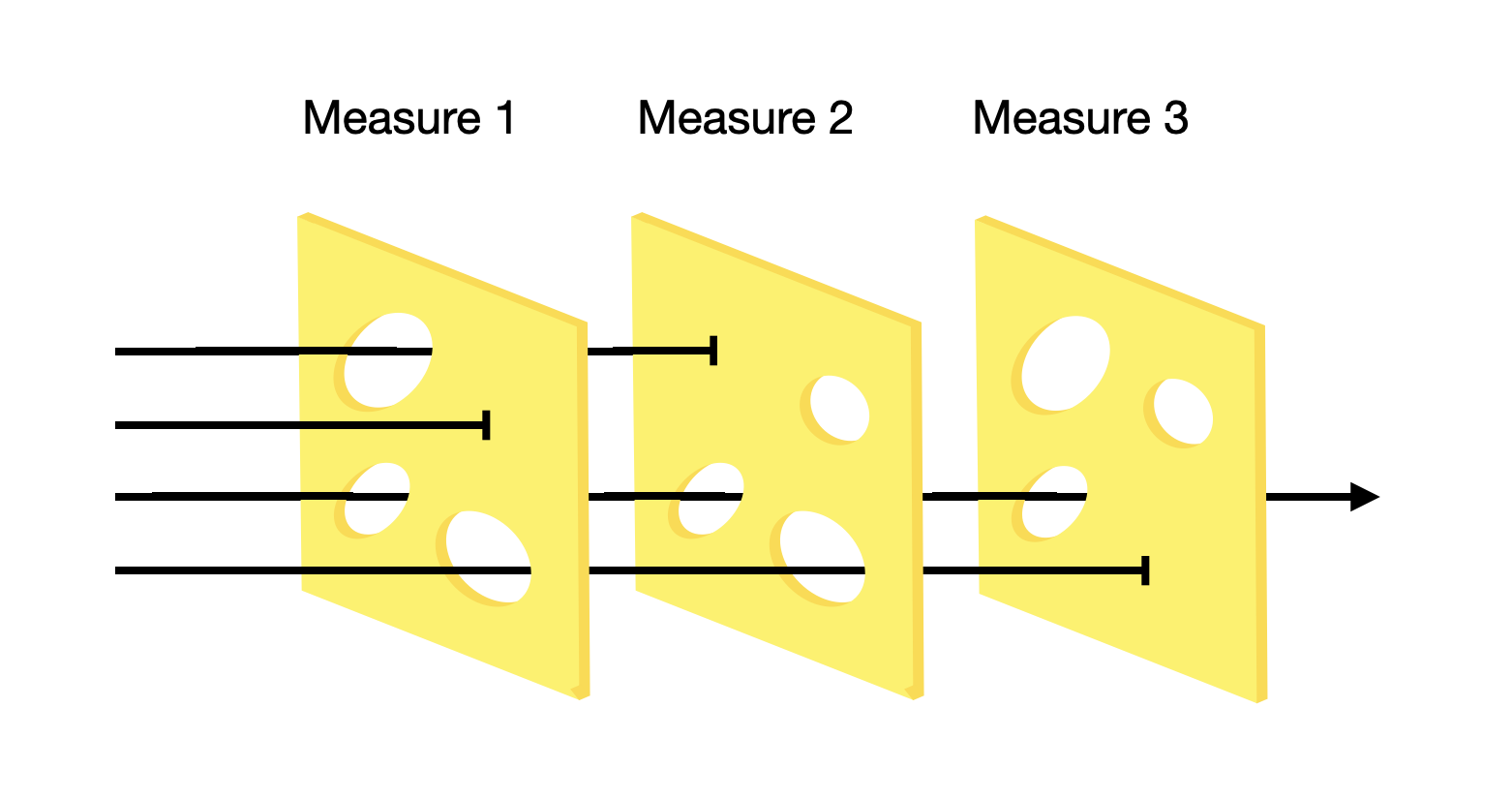
At the beginning of an outbreak of an emerging disease, there are typically no pharmaceutical interventions at hand, as the development of vaccines and therapeutics takes time. At this stage, infection control is entirely managed through NPIs. The COVID-19 pandemic provides a recent example of the numerous attempts to control infectious disease spread. The so-called “Swiss cheese model” is a useful metaphor for the idea that while none of the attempts are sufficient to control the spread of infectious disease on their own, they may nevertheless do so in combination. The fundamental idea is as follows. A pathogen needs to find its way into a susceptible host in order to infect the host and transmit to the next host. In the Swiss cheese model, every attempt to prevent this from happening is thought of as a layer of Swiss cheese with holes (the model should thus be called the Emmental cheese model, as most Swiss cheese does not have holes). The layer of cheese is capable of stopping the threat, metaphorically, but it doesn’t work sufficiently well, and the threat passes through one of the holes in the cheese layer. By combining and stacking multiple layers of the cheese, the system manages to prevent the threat from passing through all layers (Figure 4.12). Some measures like border closure are entirely government-driven. Others, such as social distancing, are largely left to individuals. Some, such as contact tracing, require a collaboration of both.
In what follows, we are going to look at some of the most common NPIs taken during the COVID-19 pandemic.
Border closure and control
One of the most significant measures taken during the COVID-19 pandemic was the closure of borders. Such closures were particularly pronounced in countries like Australia and New Zealand, where borders weren’t fully open for two years. Countries with substantial cross-border travel, especially non-tourism travel (i.e. cross-border workers), faced significant economic challenges with border closures. In addition, border closures were at times instituted in the short term, for example in the early phase of the emergence of new variants. The effect of border closures remains hard to quantify (Burns et al. 2021). Border closures are socially and economically costly, and in most cases delay the importation of cases, rather than truly prevent them.
Many countries instituted border controls over an extended period of time, rather than full border closures. This allowed countries to keep the borders open, while reducing the importation of cases. Border controls ranged from having to demonstrate a negative test and / or provide proof of vaccination, to 14-day quarantine upon arrival with multiple testings.
At this point, it’s important to make a clear distinction between quarantine and isolation. Isolation refers to the isolation of a case, i.e. where we are certain that the person is infected. The idea is that an infectious person reduces all contacts and thus cannot pass on the disease. Quarantine is a precautionary isolation, i.e. where we do not currently know for certain if the person is infected, but there is a risk, e.g. due to a possible exposure. Quarantines were first instituted in the mediterranean region during the plague epidemics in the 14th century, when ships arriving at ports were not allowed to land for 40 days. This allowed the local authorities to ensure that there was no plague on board (Tognotti 2013). Why 40 days were chosen is unknown, but the number forty gave the quarantine its name (e.g. “quarante” in French, “quaranta” in Italian).
Today, if quarantines are applied, their length is generally determined by the incubation period of the disease. Because the incubation period has some variance, quarantine periods are typically determined by the values in the distribution that are longer. For example, early estimates of the incubation period of SARS-CoV-2 were reported to be 14 days at the 99th percentile (Lauer et al. 2020), and thus the standard quarantine recommendations were generally set at 14 days. Over time, many countries reduced the duration of quarantines, or implemented a test-and-release strategy to ease the burden of quarantines. Based on available data on incubation periods, infectivity, and accuracy of tests, one can develop mathematical models to quantify the impact of quarantine duration on COVID-19 transmission (Ashcroft et al. 2021).
Closures (Schools, restaurants, events, etc.)
Most disease transmission happens where people gather and, in doing so, create many contacts for disease transmission. Closures are a strategy to prevent such gatherings by prohibiting them altogether. The most common closures during the COVID-19 pandemic were school closures, restaurant closures, and event prohibitions. While all NPIs have their costs, closures are particularly costly for everyone involved.
The effect of school closures is perhaps best studied, but nevertheless still poorly understood. Data on influenza has shown that school holidays have a pronounced effect on preventing seasonal influenza cases (Cauchemez et al. 2008). The likely reason is that during holidays, there is less mixing among children, which transmit influenza to each other and then bring it home to their households. However, the epidemiological effect of prolonged school closures remains unclear. Much depends on the contact patterns that will be established in place of the ones that are prevented by school closures. Furthermore, school closures are severely disruptive to the lives of parents, which can be very challenging particularly also for healthcare workers, whose presence is essential during health crises. Furthermore, there is now increasing evidence that school closures are detrimental to the academic advancement of children, an effect that is most pronounced in children from disadvantaged households (Engzell, Frey, and Verhagen 2021).
Test, contact tracing, isolation, and quarantine
The strategy of testing, tracing, quarantine, and isolation - TTIQ - is a bedrock of infectious disease control. The basic concept is to (i) use testing as a means to identify infected people, (ii) isolate them, (iii) trace their contacts, and (iv) quarantine them. If done perfectly, it is clear that all infection chains would be stopped, and an outbreak could be brought under control. In reality, however, there are a number of difficulties that make TTIQ less than perfect. First, it is difficult to capture all cases with testing, as mass testing is resource-intensive, and tests are typically not 100% accurate, as we’ve seen in a previous chapter. Second, tracing is even more resource-intensive, and very difficult to do thoroughly (we will discuss contact tracing in great detail in a later chapter on digital contact tracing). Lastly, depending on the type of contacts, and the incidence of the disease in the population, the number of people having to go into quarantine could be massive.
As should be obvious, the effects of contact tracing will be most pronounced in the early stages of an outbreak, when case numbers are still low (this is generally true for controlling infectious disease outbreaks: controlling small outbreaks is much easier and less costly than controlling large outbreaks). Once an outbreak starts growing rapidly, control through TTIQ becomes very difficult for the reasons just mentioned. This is why during the COVID-19 pandemic, some countries resorted to lockdowns, which are a sort of mass quarantine, where everybody is sent into precautionary isolation. Thus, TTIQ should be thought of as a potentially high-precision “lockdown”, where only a small fraction of a population must isolate in order to prevent an outbreak from growing.
The key epidemiological parameters that most strongly affect the success of TTIQ are R0, and the extent to which pre-symptomatic or fully asymptomatic transmission occurs (Fraser et al. 2004). If R0 is high, the number of contacts that have to be successfully traced and quarantined is correspondingly high as well. If there is substantial pre-symptomatic or fully asymptomatic transmission, contact tracing has to be very fast and thorough in order to be able to isolate people even without symptoms. The importance of the latter factor mustn’t be underestimated - it is likely the key factor that made SARS-CoV-1 controllable, but not SARS-CoV-2. Pre-symptomatic or fully asymptomatic transmission is virtually unknown in SARS-CoV-1, while it is very common in SARS-CoV-2. Asymptomatic infection with SARS-CoV-1 was estimated to be in the single digital percentages, and transmission from those infections rare or absent(Wilder-Smith et al. 2005). In contrast, while fully asymptomatic infection with SARS-CoV-2 remained rare (Buitrago-Garcia et al. 2022), pre-symptomatic transmission is estimated to account for about half of all transmission events (Ashcroft et al. 2020).
Masks
Masks represent a physical barrier for droplets and aerosols. There are many different types of masks, but during the pandemic, two types of masks were most often used: surgical masks, and respiratory masks. Surgical masks are loosely fitting, lightweight masks that are meant to act as a physical barrier for large droplets and sprays. Respiratory masks, on the other hand, are specifically designed to filter out airborne particles. There are different standards for respiratory masks, depending on their filtering capacity. The most commonly used standards during the COVID-19 pandemic were FFP2, a European standard, and N95, a US standard. Many governments were initially hesitant to recommend mask-wearing, likely out of a mix of concern about limited mask availability for healthcare workers, and an absence of strong evidence. In addition, while mask-wearing is relatively common in Asia, the topic of masks quickly became politicized in Europe and the US.
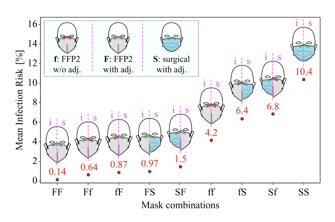
Today, the evidence for masks to reduce disease transmission is relatively strong (Howard et al. 2021). For example, research based on a physical exposure model and filter penetration experiments founds that the probability of disease transmission during a contact lasting a few minutes between an infectious individual to a susceptible individual was close to 100% when both individuals do not wear a mask; less than 30% when both wear a surgical mask; and less than 0.4% when both wear a well-fitted FFP2 mask (Bagheri et al. 2021). The risk of infection from both wearing surgical masks to both wearing well-fitted FFP2 masks is thus reduced by about factor 75. Infection risks under different assumptions of mask-wearing of the infectious and susceptible individuals are shown in Figure 4.13.
Clean indoor air
Providing clean indoor air is a key control strategy to prevent the transmission of SARS-CoV-2. Given the strong evidence for aerosol transmission, reducing the exposure to virus-laden aerosols will reduce disease transmission accordingly. Once such aerosols are in the room, they can be cleared in a number of ways, including ventilation, filtration, and disinfection. Ventilation refers to the method of replacing the air with clean fresh air, typically by creating an airflow, either mechanically or by opening windows. Filtration refers to the process of physically filtering aerosol particles. Finally, disinfection refers to the method of destroying pathogens with ultraviolet light.
The importance of clean indoor air has increased in recent years with the recognition that SARS-CoV-2 is predominantly transmitted by aerosols. Already before the COVID-19 pandemic, evidence of influenza transmission through aerosols has been growing (Cowling et al. 2013). A computational model using CO2 measurements in different rooms in a high school found that if even just half of influenza transmission is due to aerosols, good ventilation could substantially decrease disease transmission (Smieszek, Lazzari, and Salathé 2019). It’s likely that the transmission mode of other respiratory pathogens is also occurring through aerosols. Providing clean indoor air will thus likely increase in importance. Perhaps over time, clean indoor air will become the standard in the same way - and ultimately for the same reasons - that clean drinking water has become the standard for the majority of people.
Hand and surface disinfection
Hand and surface disinfection was a central piece of the COVID-19 control strategy early on in the pandemic, when fomite transmission was still assumed to play a major role. Today, we understand that fomite transmission is negligible for the transmission of SARS-CoV-2 (Rocha et al. 2021; Meister et al. 2022; Cheng et al. 2022). Nevertheless, bacterial infections, especially hospital-acquired infections (HAI), have often been shown to be reduced by improved hand hygiene (Pittet et al. 2006).
Social and physical distancing
Social and physical distancing refers to the strategy of keeping distance from others in order to limit disease transmission. The concept is largely based on the assumption of droplet transmission, which for SARS-CoV-2 is an outdated assumption, as we’ve seen previously. Nevertheless, even with aerosol transmission which can go over longer distances, close proximity transmission is still possible, and indeed common. In the early stages of the COVID-19 pandemic, most public health authorities recommended a distance of 1-2 meters. While the literature mostly uses the term social distancing, the high cost of social isolation on mental well-being during the pandemic has led to a shift of terminology, from social distancing to physical distancing. Social contacts were indeed encouraged, which can also be held digitally.