3 Epidemiological Studies
How do we know what we know in epidemiology?
Of course, this question can be asked in any field, not just epidemiology. Instead of getting bogged down in a potentially endless debate around the concept of objective truth, the goal of this chapter is to understand the different types of studies that can be conducted in epidemiology, and what level of evidence they provide. This is important so that we can make sound health decisions, either for populations at the policy level, or for individuals at the clinical level.
Historically, health practice as performed by medical experts such as doctors was not based on science, due to the simple fact that modern natural science hadn’t emerged until a few centuries ago. Even after, medical practice was largely based on standard-of-care practices combined with the personal experiences and beliefs of medical experts. Interestingly, the term evidence-based medicine is barely 30 years old. It was first used in a published manuscript in 1992, entitled “Evidence-based medicine. A new approach to teaching the practice of medicine”(Group et al. 1992). It argued that the traditional way of approaching medical decision-making - individual observations, understanding basic biological mechanisms, common sense - is insufficient, and needs to be superseded by systematic, unbiased evidence, for example on the accuracy of diagnostic tests, prognoses, and treatments.
Consequently, the question of what constitutes sufficiently strong evidence became critically important. In the past few decades, a few heuristic hierarchies of evidence have emerged that share some generalities. There is a broad consensus that the strongest form of evidence is provided by meta-analyses of randomized controlled trials (RCTs). The weakest form is expert opinion. In between, there are cohort studies, case-control studies, cross-sectional studies, and other study types. Note that it would be foolish to dismiss expert opinion, as oftentimes, expert opinion is the best level of “evidence” that is available, especially at the beginning of a newly emerging disease. It is also neither necessary to answer all questions with a randomized controlled trial, nor is it possible. As has been said before, the effect of wearing a parachute on survival rates when skydiving has never been addressed with an RCT (Smith and Pell 2003), and yet, we have a pretty solid mechanistic understanding of what the outcome would be.
Many textbooks on evidence-based medicine show a pyramid of the strength of evidence, stacking the different study types on top of each other, with RCTs at the top. We will work our way up this pyramid in this chapter. However, it’s important to be aware that this representation can be misleading as it suggests that RCTs are the strongest form of evidence in all circumstances, which is subsequently often interpreted to mean that no action should be taken on any given health issue until the data from RCTs are in. However, because RCTs are often not possible, and because they take time even when they are possible, this stance can lead to problematic situations, as we’ve seen during the COVID-19 pandemic. Early evidence on the importance of aerosol transmission and the benefits of mask-wearing were frequently dismissed because of the lack of RCTs. Put simply, RCTs were designed to assess the effect size of a particular intervention in a controlled setting. In contrast, an epidemic unfolds in a highly non-controlled setting with complex social and environmental dynamics. We thus need to understand what studies can provide what kind of evidence, rather than just blindly following a pyramid of study types, and dismissing everything that does not sit at the top of the pyramid (Greenhalgh et al. 2022). This is what this chapter is about. We will look at different study types, their strengths, and their weaknesses. We will also briefly discuss the issue of causality. In the end, you should have gained an overview of how evidence is obtained, how it can be interpreted, and in particular, you should be able to begin to read, and reason about, some of the literature describing these studies.
Before we get started, it is critical to clearly define two terms: exposure and outcome. Generally, the framework to think about this is as follows: a certain factor or condition that people are exposed to (the exposure) may or may not be associated with a certain outcome. Assessing the link between exposure and outcome is what epidemiological studies are all about. Some studies may be largely descriptive, trying to figure out how much of the exposure or the outcome is there in the first place, and if the two often occur together, i.e. if they are associated. Other studies will want to know whether the exposure truly causes the outcome.
It would be easy to think that exposure is something external that individuals are exposed to, like a virus, or an environmental factor like heat; and that outcome means health or disease. While this is often the case, it does not need to be. For example, exposure could itself be the presence of a disease. Consider, for example, a study that starts with people with a given disease, and looks at some outcome of interest (perhaps the development of another disease). Exposure can really mean anything, such as age, location, disease, behavior, etc. - any factor that may be associated with a given outcome of interest. Equally, the outcome does not need to be health or disease. It can, for example, also be a behavior, such as the decision to vaccinate, or undergo a medical procedure.
The distinction is important because, as we will see, studies will be called differently depending on whether people are selected based on the exposure, or on the outcome.
The first group of studies we will look at are observational studies. As the name suggests, observational studies are studies where we simply observe a group, and in particular the potential association of a factor (exposure) and an outcome of interest in that group. The key aspect is that we do not control this factor. Study designs where we control this factor are called experiments, and we will get to them later in the chapter.
3.1 Case reports and case series
We will work our way up the evidence hierarchy. The first level of evidence is that of case reports and case series. A case report is a report on a particular patient with a certain outcome, such as a disease. A case series is a group of similar case reports. Case reports and case series are not designed to test a hypothesis, but they can be a trigger to formulate one. We would of course be interested in what type of exposure led to the outcome. However, because participants are sampled based on the outcome only, we won’t be able to calculate any risk of exposure, let alone establish any kind of causality. Case reports are often instrumental in the early description of newly emerging diseases, and in the development of early clinical guidelines.
Among the earliest case descriptions of SARS-Cov2 - at the time named 2019 novel coronavirus (2019-nCov) - was a paper published online on January 24, 2020 (Huang et al. 2020). Describing itself as a “modest-size case series of patients admitted to hospital”, the paper described 41 cases with a laboratory-confirmed infection, including their epidemiological history and clinical presentations. It reported a disconcertingly high morbidity and mortality rate, with one-third of patients admitted to ICU care, and 6 out of 41 (15%) dying. The majority of the cases had an epidemiological link to the Huanan seafood market, and presented with fever and cough. All patients had pneumonia. These early findings were critical in alerting the world to the pandemic potential of the new virus, and developing and adjusting case definitions.
To take a more recent example, a 2022 paper on monkeypox described a case series enrolling all patients diagnosed with monkeypox at three hospitals in Spain (Tarı́n-Vicente et al. 2022). The study assessed risk factors and outcomes, and performed PCR testing. The abstract of the paper states that “data were collected by means of interviews conducted by dermatologists or specialists in sexually transmitted infections and were recorded using a standard case report form.” Nevertheless, the term case series is not used anywhere in the paper. I mention this here because many studies are case series studies, but are not designating themselves as such. To highlight the importance of case series, the paper described, among other things, how samples taken from skin lesions - a typical symptom of monkeypox - contained about three orders more viral particles than samples taken from the throat. This underlined the importance of disease transmission via skin contact, for example during sex. There are many examples like this that show how critically important case series studies are, particularly also at the beginning of an outbreak.
3.2 Ecological studies
Next are ecological studies. An ecological - or aggregate - study compares quantities of groups, rather than quantities of individuals. For example, a case series may have indicated that most people with a given disease of interest had a certain type of exposure. We could then design an ecological study, comparing different groups - for example, different countries, or different towns - by looking at their incidence of the disease, and their aggregate level of exposure. For example, research has accumulated evidence that arsenic is a carcinogen in humans. There are now numerous ecological studies linking arsenic exposure to cancer, based on aggregate data on cancer incidence and arsenic exposure (typically in drinking water). To give a concrete example, in 2016, a team of researchers compared the arsenic levels in community drinking water with the incidence of prostate cancer in different counties in the US state of Illinois (Bulka et al. 2016). They found significant dose-response, meaning that increasingly higher levels of arsenic exposure were associated with increasingly higher prostate cancer incidence in the counties.
The key benefit of ecological studies is that aggregate data are easier to obtain. It would of course be interesting to have individual-level data - and we’ll learn more about such studies later on - but it is typically quite resource-intensive to collect data on individuals. Working with aggregate data, however, creates some problems. The most egregious problem is that we are working with average values, which may hide true associations. In the case of arsenic exposure and prostate cancer incidence, it may for example be that even though the dose response exists on the level of counties, the people who developed prostate cancer in these counties have individually had very low exposure to arsenic. This problem is an example of an ecological fallacy, a kind of misinterpretation of the data that happens when you find a relationship on the aggregate level, and take it to be a relationship on the individual level.
Using the link between arsenic exposure and prostate cancer as an example, the authors of the study above state the following: “Since this study was performed on county-level data, individual-level inferences are limited. It is unknown whether prostate cancer cases in these Illinois counties were exposed to higher concentrations of arsenic than non-cases. Therefore, individual-level studies of prostate cancer incidence and arsenic exposure are needed to confirm the associations observed in this analysis.” This shows that the authors are clearly aware of the ecological fallacy, and provide ways to address it. Being clear about the limitations of your study, and thinking about future ways to resolve those limitations, is one of the hallmarks of good science.
Let’s use a simple example. Say we’re performing an ecological study by comparing the average exposure with disease incidence in four different groups. It turns out that the average exposure is positively correlated with the disease incidence at the level of groups. Can we conclude that higher exposure means higher disease probability in individuals? No, that would be falling victim to the ecological fallacy. Yes, groups with higher exposure have higher incidence - but we cannot interpret that correlation on the aggregate level to mean that the relationship is also there on the individual level. To see why, let’s assume that we all of a sudden get access to individual-level data. In Figure 3.2, we plot the exposure of all individuals, vertically separated by group.
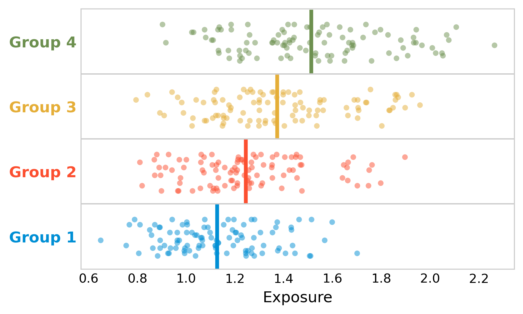
In each group, there are 100 people. The disease incidence per group is as follows: 5% in group 1, 10% in group 2, 15% in group 3, and 20% in group 4. The ecological analysis thus tells us that the higher the exposure, the higher the incidence - at the group level.
To see whether this is true on the individual level as well, we will now plot the figure again, but this time, we are going to highlight the people who have the disease. Figure 3.3 shows that diseased individuals appear to be clustered around low to intermediary value of exposure. Indeed, a statistical test would show that there is no difference in the mean exposure of diseased and non-diseased.
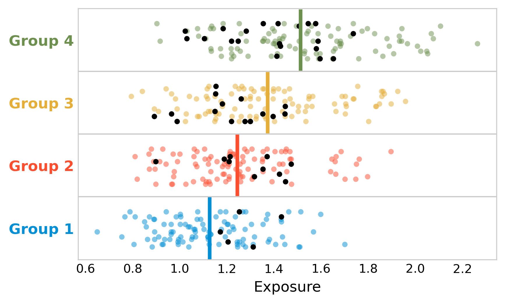
What is going on here? The ecological study shows that indeed, the disease incidence was higher in the groups that had higher exposure - there is nothing wrong with this claim. But looking at the individual data, it’s likely that the exposure is not the driving factor for disease incidence. There may be other factors that contribute to some groups having higher disease incidence than others, and that also correlate with exposure. For example, it could be that our hypothetical disease is strongly influenced by age, and that the groups with the highest exposure also happen to be associated with the highest average age. In addition, bias may be at play, whereby people with the disease preferentially move to group 3 or group 4, perhaps because the healthcare system is better. It’s common to try and control for such factors in a study, if the corresponding data is available. For example, the arsenic study authors write in their discussion that “it is possible that confounding may have biased our results”, and that they “adjusted for age by standardizing, and further controlled for county-level covariates including race/ethnicity, socioeconomic status, and private well use”.
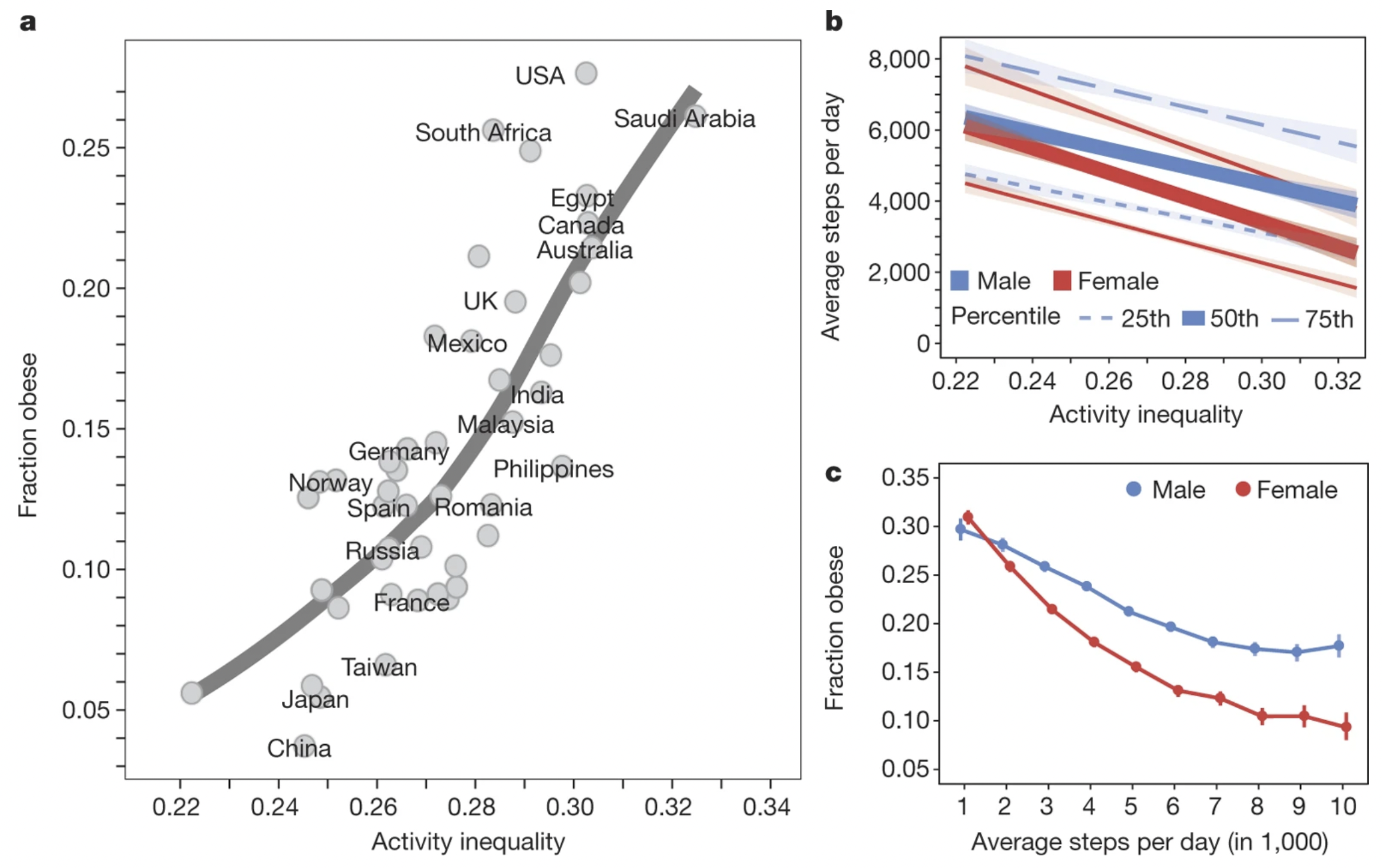
Ecological studies are very common in digital health studies. The widespread use of wearable devices, for example, enables data collection on a large scale, which is sometimes made available to researchers in aggregated format. A well-known example is a large-scale study on physical activity, based on data from a smartphone app used to track physical activity (Althoff et al. 2017). The study analyzed 68 million days of physical activity for 717,527 people in 111 countries, and calculated an activity inequality index which measures how equally the activity is distributed in the population sample from a given country. The results revealed a strong association between physical inactivity (Figure 3.4), and that at the aggregate population level, physical inequality is a better predictor of obesity than average activity volume. We will return to digital health studies later in the book with a dedicated chapter.
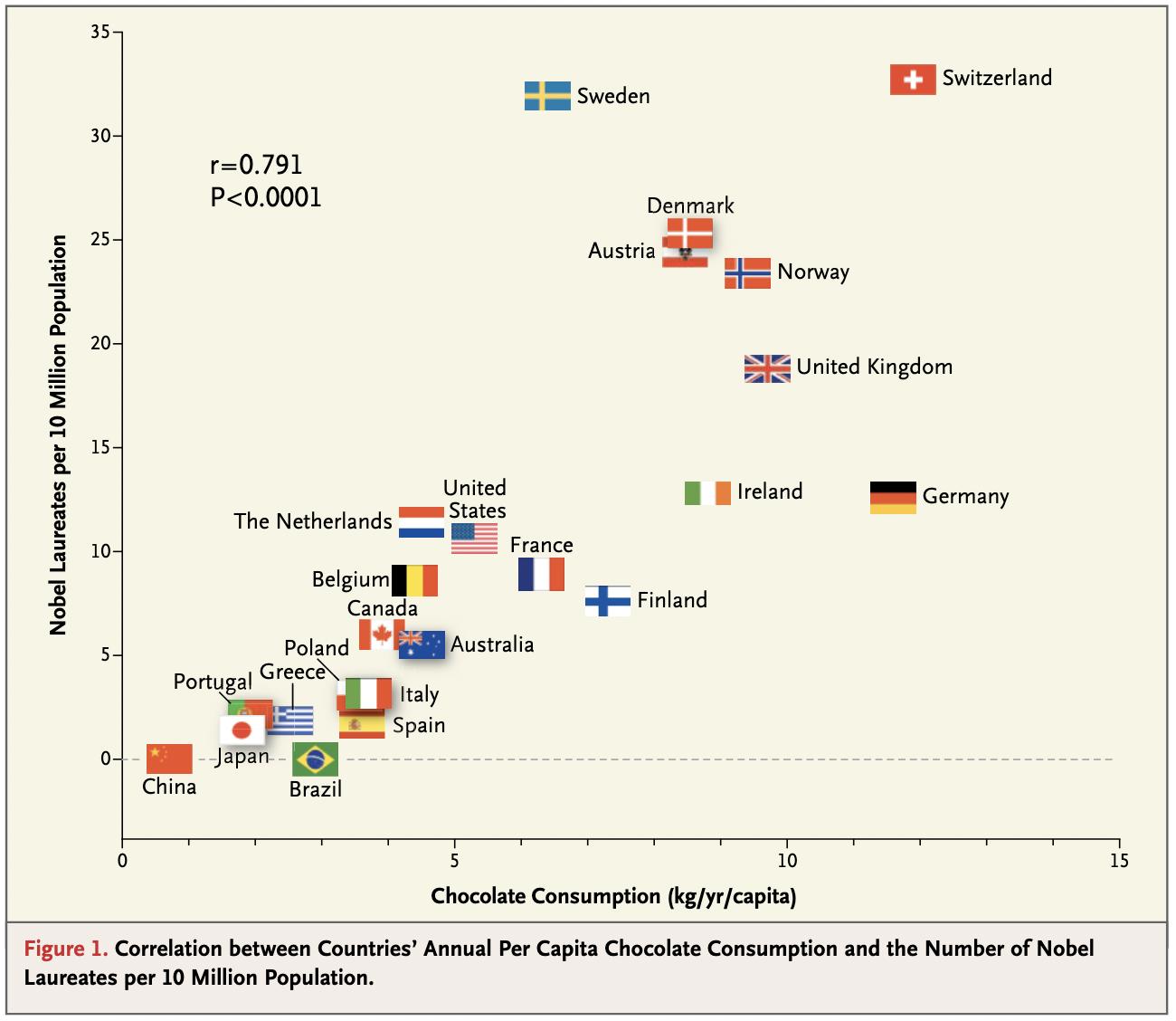
One of the most amusing ecological fallacies was published - tongue in cheek - in the New England Journal of Medicine in 2012 (Messerli 2012). In the paper, the author argues that chocolate consumption positively and significantly correlates with Nobel laureates per capita (Figure 3.5), concluding that “it seems most likely that in a dose-dependent way, chocolate intake provides the abundant fertile ground needed for the sprouting of Nobel laureates.” Once again, the key point is that we do not know whether individual Nobel laureates ate more chocolate than other individuals. The author concludes by saying that “these findings are hypothesis-generating only and will have to be tested in a prospective, randomized trial.” Needless to say, such a trial is not possible, but the notion that an ecological study provides ground to move on to other study designs that can provide stronger forms of evidence is spot on.
3.3 Cross-sectional studies
Cross-sectional studies are studies where data is collected at a given point in time (hence the term). Because cross-sectional studies are snapshots at a point in time, they are typically not able to say anything about incidence, which requires time. Cross-sectional studies can mostly assess prevalence, which is why they are often called prevalence studies. Another name that is used for cross-sectional studies is survey studies, as many studies using surveys collect data at one point in time. The main benefit is the same as that of ecological studies: they are relatively inexpensive to conduct. Like case series and ecological studies, they can be important in generating hypotheses, and in helping describe newly emerging diseases, or the consequences thereof.
To take a recent example, cross-sectional studies were used early in the COVID-19 pandemic to assess students’ mental health. One study conducted an online survey on mental health among undergraduate and graduate students of Texas A&M University in the first half of May 2020 (Wang et al. 2020). The survey found alarmingly high proportions of the 2,031 respondents showing depression (48.14%), anxiety (38.48%), and/or suicidal thoughts (18.04%). As with most observational studies, a key problem is bias. Respondents to surveys may self-select based on the interest of the survey (selection bias). In the mental health case, it’s possible that participants with mental health problems were more interested in participating in research about mental health. Further, because cross-sectional studies are snapshots, it’s often difficult to compare these numbers with numbers that would have been generated, say, one year before the pandemic.
The opposite of a cross-sectional study is a longitudinal study, where data are collected at multiple time points. To stick with the topic of mental health during the COVID-19 pandemic, numerous longitudinal studies looked at how mental health evolved over time, and some were able to compare the results to pre-pandemic levels. For example, data from multiple surveys on mental health were compared with mental health data from the UK household longitudinal study collected between 2017 and 2019 (Daly, Sutin, and Robinson 2022), providing evidence that mental health deteriorated in the first half of 2020. More recent studies suggest that throughout the pandemic, mental health trajectories have continued to deviate from expected pre-pandemic levels (Wiedemann et al. 2022).
3.4 Case-control studies
Case-control studies are studies that look at groups that differ in the outcome. Oftentimes, case-control studies compare a group with a disease to a group that does not have the disease (however, recall that the outcome does not necessarily need to be a disease). A good case-control study design compares two groups that are identical except for the outcome of interest. It then looks at the levels of exposure in the case group, and in the control group. The analysis should be able to show whether the exposure is associated with the outcome, and how. For example, assuming a binary exposure (present or absent) and a binary outcome, we’d expect our case group to have been exposed more frequently than the control group.
In order to quantify the association between exposure and outcome, we can calculate an odds ratio. Imagine we designed a case-control study where we looked at the presence or absence of a disease as an outcome. We have two groups, patients with the disease (the case group), and an otherwise similar group without the disease (the control group). Starting from this, we assess how many in each group have been exposed. Let’s say the result of this assessment is the following table:
| Disease | No disease | |
|---|---|---|
| Exposed | 90 | 150 |
| Not exposed | 30 | 570 |
The odds ratio represents the odds that the disease occurred when exposed, relative to the odds that the disease did occur when not exposed. The odds that the disease occurred when exposed is \(\frac{90}{150} = 0.6\); the odds that the disease occurred when not exposed is \(\frac{30}{570} = 0.0526\). The odds ratio is thus \(\frac{0.6}{0.0526} = 11.4\). Such a high odds ratio means that the exposure is strongly associated with the disease. Note that from this information alone, we cannot establish causality, no matter how high the odds ratio. The odds ratio simply says that the odds are over 11 times higher of developing the disease when the exposure is present. There could for example still be an unknown confounding factor that causes the disease, and that is strongly associated with the exposure as well.
In reality, because our study participants are always just a sample of the total population from which they were drawn, we will need to report results like odds ratios with a confidence interval. A 95% confidence interval for the odds ratio can be calculated as
\[95\%\ CI = OR * e^{\pm 1.96 \sqrt{\frac{1}{N_{D|E}}+\frac{1}{N_{D|¬E}}+\frac{1}{N_{¬D|E}}+\frac{1}{N_{¬D|¬E}}}}\]
where \(N_{D|E}\), \(N_{D|¬E}\), \(N_{¬D|E}\), and \(N_{¬D|¬E}\) are the numbers for the contingency table. Thus, for the values above, we would report the odds ratio as 11.4 (95% CI, 7.3 - 17.9).
Case-control studies are very widespread in epidemiology. Here are just a few examples of influential case-control studies. In 2007, a case-control study of Human Papilloma Virus (HPV) and oropharyngeal cancer (a cancer in the back of the throat) reported an odds ratio of 32.2 (95% CI, 14.6 to 71.3) for oropharyngeal cancer and seropositivity for the HPV-16 L1 capsid protein (D’Souza et al. 2007), which is a measure of lifetime HPV-16 exposure. HPV-16 is one of many types of HPV that is now well-known to be a major cause of oropharyngeal and cervical cancers. In 2016, a case-control study of Guillain-Barré Syndrome, an autoimmune disorder leading to muscle weakness, and the Zika virus infection reported an odds ratio of 59.7 (95% CI, 10.4 to ∞) for Guillain-Barré syndrome and Zika virus IgM and/or IgG positivity (Cao-Lormeau et al. 2016), a strong signal for recent Zika virus infection. Going back further in time, some of the first strong clues about the link between smoking and lung cancer came from a case-control study (even though it wasn’t called that at the time) in England. The researchers recruited 709 lung cancer patients, and 709 otherwise comparable non-cancer patients, and looked at the number of cigarettes smoked (Doll and Hill 1950). While the use of odds ratios was uncommon at the time, the data was convincing enough for them to conclude “that there is a real association between carcinoma of the lung and smoking“.
One of the key advantages of case-control studies is that one can start with the outcome, and look back. As we’ll see shortly, starting with the exposure and looking at outcomes in the future, as is done in many cohort studies, can take a long time. Another advantage is that by starting with the outcome, one can also study rare outcomes. Even if a disease is rare - such as the Guillain-Barré Syndrome mentioned above - a case-control study can simply start with all or most of the cases, even if the disease itself is rare. This is particularly important at the beginning of an outbreak of a newly emerging disease, and one of the main reasons why case-control studies are often performed in the early stages of building up evidence to support a link between an exposure and an outcome.
The key difficulty, on the other hand, is that bias can be difficult to avoid. The two types of bias that are particularly pertinent to case-control studies are selection bias and recall bias. Selection bias can occur when cases and controls are selected based on a factor related to exposure. For cases, this would mean that the selected cases are not representative of all cases; for controls, this would mean that the selected controls are not representative of the larger population. If we start with outcomes, and want to see if there is an effect of exposure on outcome, as we do in case-control studies, it is obviously highly problematic to select individuals based on exposure, or related factors. Recall bias is a type of information bias; it occurs when cases are more likely to recall and report exposure than the control individuals. This can easily lead to an underestimate of exposure in the control group, and therefore in the claim of having found an association between exposure and outcome when none exists.
3.5 Cohort studies
The last type of observational study we will discuss is the cohort study. Cohort studies are studies that start with different levels of exposure, and try to see if the outcome of interest is associated with the levels of exposure. The goal - understanding if there is an association between exposure and outcome - is thus the same as in a case-control study; the key difference is that the cohort starts by comparing different levels of exposure, while the case-control study starts by comparing different levels of outcome.
Notice that a case-control study, which starts with different groups of outcome, is necessarily a retrospective study, i.e. going back in time. The outcome is always the endpoint, thus you cannot design a prospective case-control study. With cohorts, that is different. Cohorts start with different groups of exposure. This could be now, and we can plan the cohort to observe the outcomes in the future. This is called a prospective cohort. However, we can also find different groups of exposure in the past, and see how the outcome developed. This would be called a retrospective cohort. Unless specified otherwise, when I use the simple term cohort, I mean a prospective cohort.
Both retrospective cohorts and case-control studies look backward in time. It’s thus easy to confuse them. The key difference is that in case-control studies, subjects are selected based on an outcome, with the goal of identifying differences in exposure, whereas in retrospective cohorts, subjects are selected based on exposure, with the goal of identifying differences in outcome.
In the most straightforward study design, we begin with two groups, one exposed and one not exposed, and follow the individuals for some time, after which some will have developed the disease. We can then again create a disease vs exposure table, as we did before in the section on case-control studies. In fact, to simplify things, let’s assume that we obtain the same numbers in our hypothetical cohort as those that we used in our hypothetical case-control study:
| Disease | No disease | |
|---|---|---|
| Exposed | 90 | 150 |
| Not exposed | 30 | 570 |
From this, we can now calculate the relative risk, or risk ratio. You may now ask, why relative risk, instead of odds ratio, as we did for the case-control study? We’ll get back to that question shortly.
The relative risk is the risk of developing the disease when exposed, relative to the risk of developing the disease when not exposed. The latter is also called baseline risk. The disease risk when exposed in this example is \(\frac{90}{90+150} = 0.375\). This corresponds to the probability that you get the disease, given exposure, \(P(D|E)\). The baseline risk is \(\frac{30}{30 + 570} = 0.05\), which corresponds to the probability that you get the disease, given no exposure, \(P(D|¬E)\). The relative risk is simply:
\[Relative\ risk = \frac{P(D|E)}{P(D|¬E)}\]
With our numbers, that corresponds to \(\frac{0.375}{0.05}\), which is 7.5.
As with odds ratios, risk ratios should be reported with a confidence interval. A 95% confidence interval for the risk ratio can be calculated as
\[95\%\ CI = RR * e^{\pm 1.96 \sqrt{\frac{1-P(D|E)}{N_{D|E}} + \frac{1-P(D|¬E)}{N_{D|¬E}}}}\]
Thus, for the values above, we would report the risk ratio as 7.5 (95% CI, 5.1 - 11).
In the section on case-control studies above, we calculated the odds ratio, instead of the relative risk, which was 11.4. You will recall from the discussion about likelihood ratios in Chapter 2 that odds can easily be calculated from probabilities, and vice versa, as \(odds = \frac{probability}{1-probability}\). Thus, we can calculate the odds ratio in terms of risks (which correspond to probabilities) as follows:
\[Odds\ ratio = \frac {\frac{P(D|E)}{1-P(D|E)}}{\frac{P(D|¬E)}{1-P(D|¬E)}}\]
which also gives us 11.4.
Given a disease vs exposure contingency table, we can calculate both odds ratio and relative risk. For cohorts, that is fine. But for case-control studies, calculating a risk ratio makes no sense. Why is that? It goes back to the definition of risk (probability) and odds. In the context of these studies, we are interested in the association of exposure and outcome, assuming that the exposure influences the outcome. Thus, when we start from the exposure, as we do in cohorts, it makes sense to talk about risk, or probability, of the outcome. But when we start from the outcome, as we do in case-control studies, it makes no sense to talk about the risk of outcome: we began at the outcome, after all. That’s why we use the odds ratio instead. Note that in the case of a retrospective cohort study, we could use both.
How does one interpret the different values of odds ratio and relative risk? If you look again at the equations for relative risk and odds ratio above, you’ll notice that if \(P(D|E)\) and \(P(D|¬E)\) are small, then the two terms are almost identical (because of the division by ~1). This is the case in rare diseases, where the prevalence is very low. Generally, the odds ratio will always be greater than the relative risk, but we can see in Figure 3.6 how the odds ratio relates to relative risk based on the baseline risk \(P(D|¬E)\).
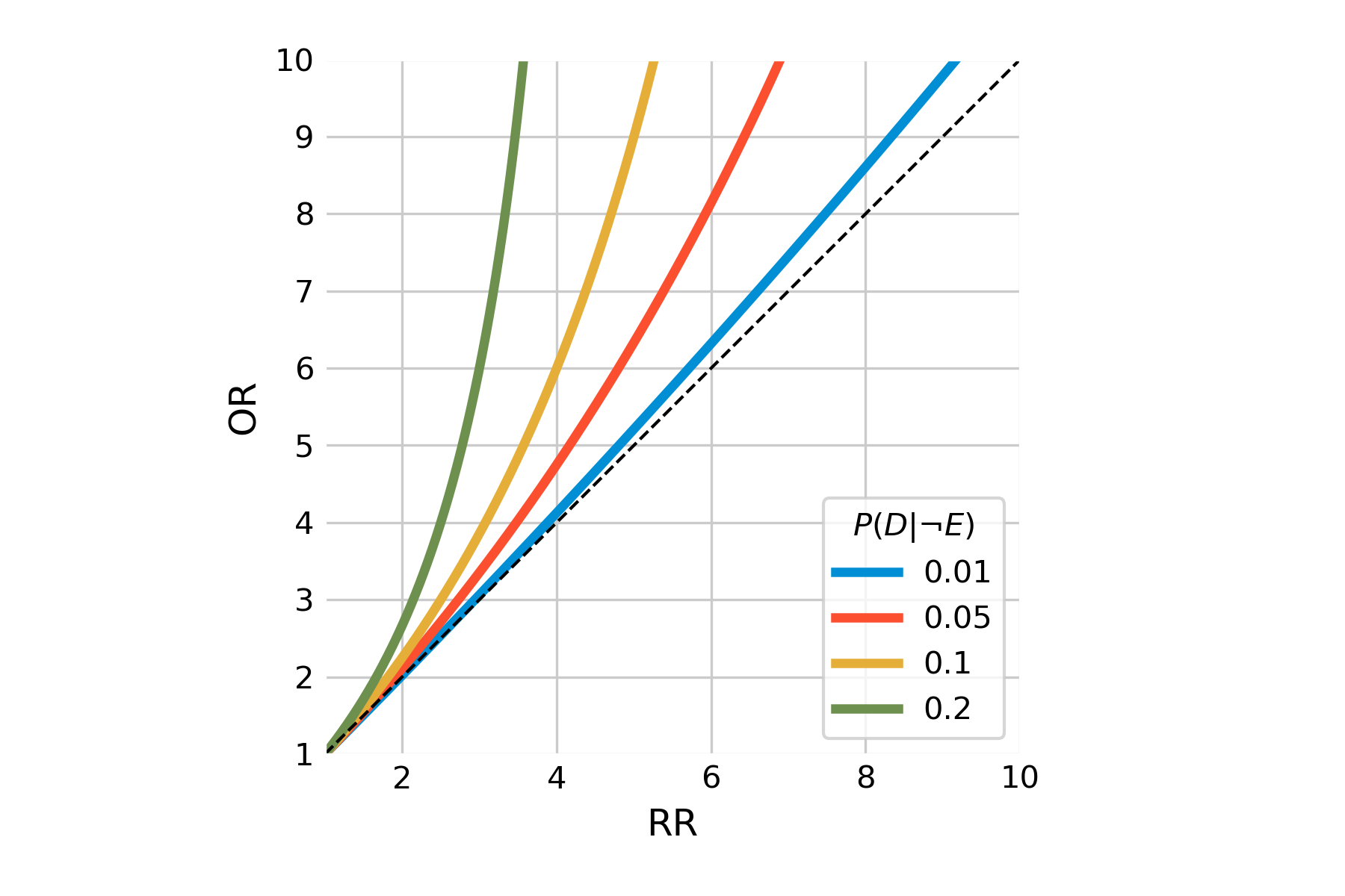
We can easily calculate the odds ratio from the relative risk, because
\[Odds\ ratio = \frac {\frac{P(D|E)}{1-P(D|E)}}{\frac{P(D|¬E)}{1-P(D|¬E)}} \] \[= \frac{P(D|E)}{1-P(D|E)} * \frac{1-P(D|¬E)}{P(D|¬E)}\\\] \[= \frac{P(D|E)}{P(D|¬E)} * \frac{1-P(D|¬E)}{1-P(D|E)}\\\] \[= relative\ risk * \frac{1-P(D|¬E)}{1-P(D|E)}\]
We can confirm that \(11.4 = 7.5 * \frac{1-0.05}{1-0.375}\).
The biggest advantage of (prospective) cohorts is that cohort study designers can specifically determine what data should be gathered, and how. This is not possible for case-control studies, or retrospective cohorts, where the data has already been collected. The downside is that cohorts are difficult for diseases that take a long time to develop, or are rare (or both). On the other hand, because cohorts start from the exposure, it is a study design that is well suited for rare exposures.
Cohorts can also look at multiple outcomes. Oftentimes, cohorts are based on people being part of the same group, such as a geographic location, and particular professional position, or being born in the same year (birth cohort). Well-designed, long-term cohorts are expensive, but have been providing tremendously valuable insights into various public health aspects. For example, the Framingham heart study is a cohort that began in Framingham, Massachusetts (US) in 1948 in order to better understand the development and risk factors of cardiovascular diseases (Mahmooda et al. 2014). The Nurses’ Health study is a cohort starting in 1976, recruiting female registered nurses with the goal of studying contraceptive use, smoking, cancer, and cardiovascular disease (Bao et al. 2016). Both studies have since then continuously expanded in scope, enrolling hundreds of thousands of participants, and resulting in thousands of scientific publications on various exposure / outcome associations. Another famous long-term cohort is the British Doctor’s study, which ran from 1951 to 2001, and provided critical evidence for the detrimental health effects of smoking (Doll and Hill 1954). It was launched after the publication of the case-control study mentioned above.
3.6 Randomized controlled trials
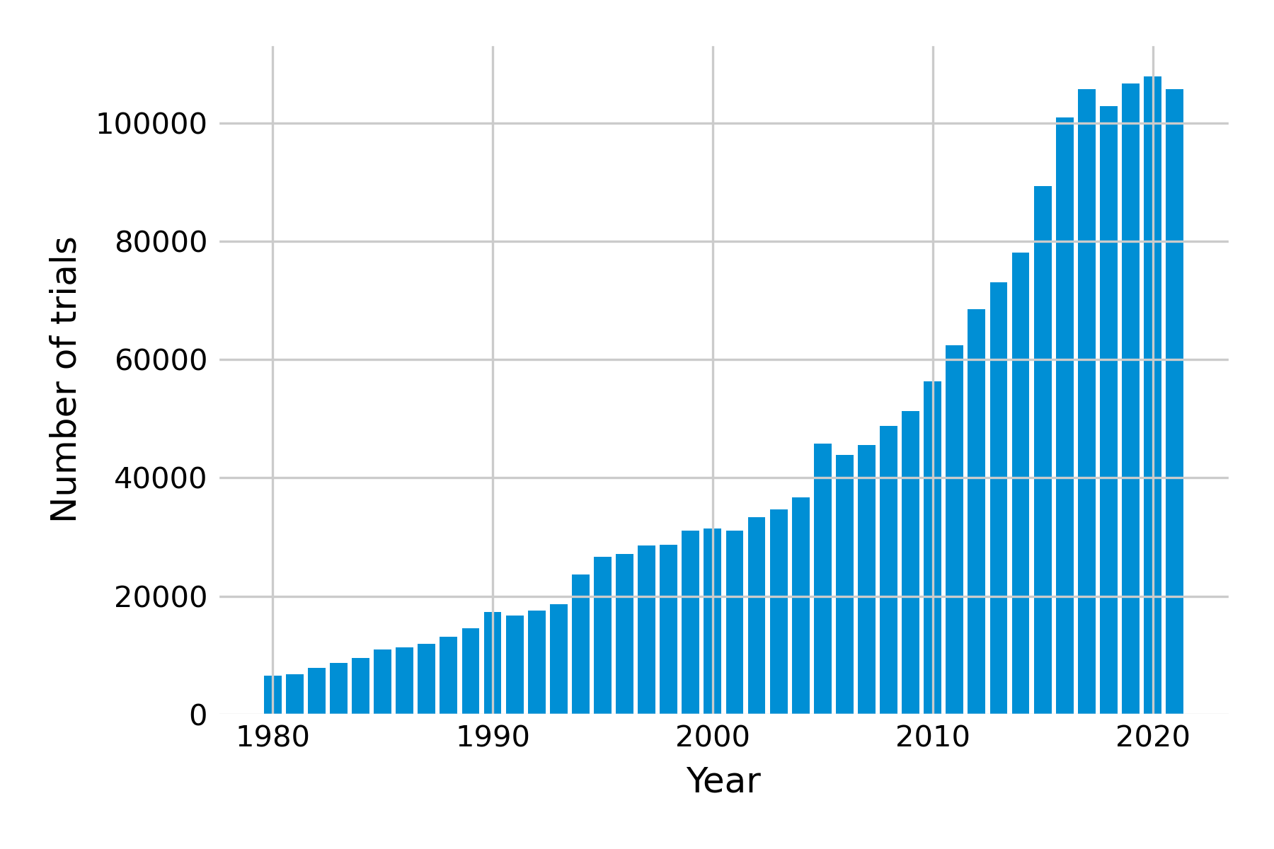
We now leave the realm of observational studies and move towards experimental studies. Here, we don’t just observe the exposure; we control it with interventions. Studies that experimentally test interventions are called trials. These types of studies have become increasingly common (Figure 3.7). Experimentally controlling interventions is obviously only possible if the deliberate application of the intervention is ethically justifiable. For example, it would be highly unethical for researchers to ask people to start to smoke, or to deliberately engage in unsafe sex, just so one can obtain high-quality evidence. Thus, in many trials, the goal is to assess a type of intervention where one can assume that it is relatively safe. We’ll talk more about arriving at that assumption later on.
The state-of-the-art study design is the randomized controlled trial. In this study design, participants are assigned randomly to one of two (or more) groups. In the classical scenario of two groups, one group receives the intervention, and the other doesn’t. The point of the randomization is to avoid confounding. Ideally, nobody knows in which group they are, in order to avoid any effects that could be associated with knowing which group one is in. This is called blinding, or masking. In a single-blind trial, only the participants are unaware of their group assignment. In a double-blind trial, neither the participants not the researchers know the group assignments during the trial. An open label trial is a study where there is no blinding. Blinding is easiest with placebo, but depending on the intervention under study, placebos may not always be available. For example, when a study assesses the efficacy of a behavioral intervention, it may be difficult to hide group assignments. In general, with more and more data available to individuals directly - for example through sensors, smart watches, and other devices - it may become increasingly difficult to ensure full blinding.
To take a recent and much-discussed example, let us take a look at the studies that evaluated the efficacy of COVID-19 vaccines. The first study to be published after peer-review looked at the efficacy of the Astrazeneca (ChAdOx1) vaccine (Voysey et al. 2021). The authors write in the abstract, “This analysis includes data from four ongoing blinded, randomised, controlled trials done across the UK, Brazil, and South Africa. Participants aged 18 years and older were randomly assigned (1:1) to ChAdOx1 nCoV-19 vaccine or control”. They later say that “vaccine efficacy was calculated as 1 − relative risk”. Without going into the statistical details, we already have a basic understanding from these statements how the trial was set up and evaluated.
The second study looked at the efficacy of the Pfizer-BioNTech (BNT162b2) mRNA vaccine (Polack et al. 2020). The authors write, “In an ongoing multinational, placebo-controlled, observer-blinded, pivotal efficacy trial, we randomly assigned persons 16 years of age or older in a 1:1 ratio to receive two doses, 21 days apart, of either placebo or the BNT162b2 vaccine candidate (30 μg per dose).” Observer-blinded here means that everyone was blinded. Further down in the article, they write that “Vaccine efficacy was estimated by 100×(1−IRR), where IRR is the calculated ratio of confirmed cases of Covid-19 illness per 1000 person-years of follow-up in the active vaccine group to the corresponding illness rate in the placebo group”. Without going into the details of why the rate was expressed per 1000 person-years, the idea here is exactly the same as in the first study; IRR here corresponds to the risk ratio as defined above, i.e. \(\frac{P(D|E)}{P(D|¬E)}\).
The third study looked at the efficacy of the Moderna (mRNA-1273) mRNA vaccine (Baden et al. 2021). The authors write, “This phase 3 randomized, observer-blinded, placebo-controlled trial was conducted at 99 centers across the United States. Persons at high risk for SARS-CoV-2 infection or its complications were randomly assigned in a 1:1 ratio to receive two intramuscular injections of mRNA-1273 (100 μg) or placebo 28 days apart”. Further down, they write that “Vaccine efficacy was defined as the percentage reduction in the hazard ratio for the primary end point (mRNA-1273 vs. placebo)”, which is not quite correct; the reduction is in the hazard, not the hazard ratio. The authors clarify this in the supplementary appendix, where they state that “Vaccine efficacy (VE) is defined as the percent reduction in the hazard, i.e. one minus the hazard ratio (HR, mRNA 1273 vs. placebo).“ Note the primary endpoint refers to the effect that the study tries to measure. Here, the authors use a hazard ratio, instead of a risk ratio. These two are quite similar, but risk usually refers to a cumulative risk of a certain outcome occurring over the entire study period, while hazard refers to the instantaneous risk of the outcome at any point in time.
Let’s take these three studies to introduce the concept of validity. When designing a study such as a randomized controlled trial, we need to ask ourselves how valid our findings are. Internal validity refers to the strength of the conclusions in the study. In the case of a randomized controlled trial, internal validity refers to our ability to establish causality between the exposure and the outcome, which depends on study design, removal of bias, appropriate blinding, and other factors. External validity refers to the extent to which our results can be generalized beyond the study setting. An important factor to increase external validity is to ensure diverse, representative study populations. When it comes to assessing how well a treatment works, these two concepts are mapped onto the terms efficacy and effectiveness. You will note that in the discussions of the vaccine trials above, all studies referred to vaccine efficacy. They did that because efficacy refers to how well the vaccine worked in the study. Later studies assessed how well the vaccine worked out in the real world, and these studies always refer to vaccine effectiveness (Lau et al. 2023). The two can be different, because trials are often done under highly controlled conditions that the real world won’t provide.
We can see from these three examples that the concepts discussed in this chapter already help us understand the abstracts of very important studies. Randomized controlled trials are indeed the gold standard to evaluate how well an intervention works. So why don’t we always go straight to randomized-controlled trials, provided we have the resources? We touched on one of the answers above, which is that the intervention must be ethically justifiable. In the case of pharmacological interventions such as drugs or vaccines, there is a framework in place to guide the decision. The third vaccine study that we just discussed alluded to this briefly, by mentioning that the trial was a phase 3 trial.
The development of medical interventions typically goes through a number of stages2. The earliest stage is called the pre-clinical phase, which means that a candidate intervention is tested outside of the human, either in vitro, or in animals. Phase I is the phase where the intervention is for the first time tested in humans, typically in small groups of usually dozens of participants. The goal is not to evaluate efficacy - phase 1 studies are often too small for that anyways - but rather to evaluate tolerability and safety, and the optimal dosing with respect to side effects. If an intervention appears safe in certain doses, it can then be evaluated for initial efficacy and continued safety in a phase 2 trial, which is larger (usually hundreds of participants). This is a kind of pilot trial to demonstrate if the intervention has the desired beneficial effects without serious negative side effects, and to identify the dose with the best benefit / risk ratio. About half of the studies get past this stage. Those who do, can enter phase 3, which is now the full efficacy and safety assessment of the intervention. Again about half of the phase 3 trials eventually make it to market (Wouters, McKee, and Luyten 2020). Of course, the intervention first needs to go to the health authorities for regulatory approval before it can be offered on the market.
Going through all the phases takes time and resources. Given that most of the intervention candidates fail, the costs for an intervention to successfully pass all phases until regulatory approval are estimated to be on average 1.3 Billion US dollars. A large part of those costs are the costs of failed trials. But the system in place ensures that drugs that are available to patients on the market are generally quite safe. Nevertheless, in order to ensure continued safety, so-called phase 4 studies, or post-marketing studies, assess how the intervention performs in the real world. Once an intervention is prescribed to millions of people, infrequent side effects that were missed in the previous phases may manifest themselves. In rare cases, reanalysis of data has shown that a drug has negative side effects that were not seen, or not considered problematic in the original analysis before approval. This is a type of pharmacovigilance that can sometimes take years or even decades. In some cases, drugs have been recalled that had been on the market for many decades (Safer, Zito, and Gardner 2001). In other cases, some drugs (Topol 2004) were believed to cause tens of thousands of deaths (Graham et al. 2005) while on the market, because the drug was prescribed to tens of millions before recall. One of the most well-known examples is rofecoxib (most commonly sold under the brand name Vioxx), which was prescribed to over 80 million people worldwide before being pulled from the market. Thankfully, these are rare events, but they go to show the extreme rigor that needs to be applied in conducting and analyzing all studies, from the original case report all the way to the final randomized controlled trial before market approval, and pharmacovigilance studies afterward.
Cohorts and trials, which can provide some of the strongest epidemiological evidence, are resource-intensive. Digitization can help address this issue, and we’ll get back to that topic in a later chapter on digital cohorts and trials.
3.7 Systematic reviews and meta-analyses
While randomized controlled trials are the gold standard for demonstrating whether an intervention works as expected, each study nevertheless provides only one data point - for example, reporting a relative risk. Over time, multiple studies on a given association between exposure and outcome may appear, with different results. The evidence from such studies can be collected, analyzed, and synthesized in systematic reviews. As the name suggests, systematic reviews systematically select and assess the studies for a given topic, minimizing biases and errors. Systematic reviews can be done with different types of studies, not just randomized controlled trials.
Systematic reviews in health research emerged in the 1980s. The key problem with “non-systematic” reviews is that the inclusion of studies and their results is highly subjective, entirely left to the authors’ liking. Consequently, the conclusions of non-systematic reviews may be highly biased. Systematic reviews address this shortcoming by following a systematic process. This includes, among other things, the definition of clear inclusion and exclusion criteria, the preparation of a study protocol, the assessment of risks and biases, and the analysis of the data. A reader should in principle be able to reproduce the review and come to the same conclusions.
If the studies are similar enough, and the corresponding data available, a statistical pooling of the results - a so-called meta-analysis - may be done to determine the size of the effect, reported over multiple studies. The overall goal of such a meta-analysis is to produce a single estimate of the effect of the intervention. Meta-analyses weigh studies according to their size - or rather by the inverse of the variance, which itself relates closely to trial size. The results of the different studies can be shown in a so-called forest plot. An example is shown in Figure 3.8, which shows the risk ratios - with their 95% confidence intervals - of studies investigating the mortality-preventing effect of beta‐blockers after myocardial infarction.
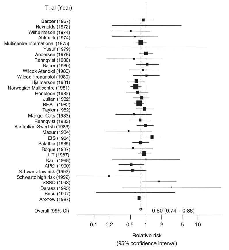
The plot also shows the mean and confidence interval of the combined relative risk, showing a 20% reduction in risk. One can see from the plot that some individual studies showed an increase in risk, but also that they tended to be smaller.
A meta-analysis can also be done in a temporally cumulative fashion. Note that in Figure 3.8, the studies span the time period from 1967 to 1997. What would the mean risk have been after every new study? In other words, if the meta-analysis had been performed upon publication of every single new study, at what point could we have had enough evidence showing that beta blockers reduce the risk of mortality after a heart attack? This is the goal of a cumulative meta-analysis, whose corresponding forest plot is shown in Figure 3.9:
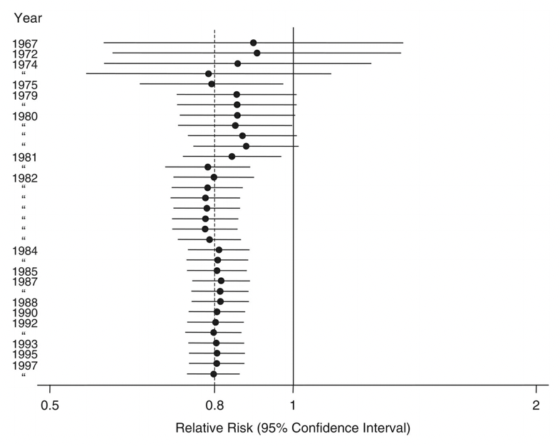
The cumulative forest plot clearly shows that a significant risk reduction became evident in 1981, which also raises ethical questions about the need for further studies even a decade later, in which people were given a placebo instead of a beta-blocker, despite the clear evidence of the latter’s beneficial effect.
Indeed, Figure 3.9 raises general questions about the timing of the studies, and the drawing of conclusions. Studies take time to plan, and to execute. Publication through a peer review process can also take a lot of time. Once a study is published, the time until its inclusion in a systematic review or meta-analysis can be significant. Meta-analyses themselves can take a long time to produce and publish. After their publication, they are rarely updated. Because of all of these delays, systematic reviews may quickly become inaccurate. Given that such reviews are strongly influencing health guidelines, such inaccuracies can have serious negative consequences. In recent years, the emergence of living systematic reviews has tried to address these challenges. Cochrane, an international network of researchers that performs systematic reviews, defines living systematic reviews as reviews which are “continually updated, incorporating relevant new evidence as it becomes available”5. In general, the question of how digital technology can help with the (semi-)automated assessment of new published studies - given the massive growth in recent decades - is highly relevant to digital epidemiology. For example, a recent review looked at deep learning language models to support the creation of living systematic reviews for the COVID-19 literature (Knafou et al. 2023) and found that modern natural language processing (NLP) approaches can serve as alternative assistants for the curation of systematic living reviews. It’s quite likely that future versions of large language models like GPT-3 and its descendants like ChatGPT will be able to systematically assess and summarize with only very limited input from experts.
3.8 Causal inference
We’ve now worked our way up the “hierarchy of evidence” pyramid. Once again, we should remind ourselves that the stacking of the pyramid should not be taken too figuratively - all levels of hierarchy can provide useful information, and all study types have both strengths and weaknesses. A core reason why RCTs are near the top of the pyramid is that they are the only study type that can establish causality. At least, that is what most textbooks would make you believe. And indeed, while RCTs are a well-established method to establish causality, observational studies do not have to be completely silent on the topic. Let’s briefly look at why causality is important, why the RCT design allows us to establish causality, and why observational studies have in the past decades begun to slowly emerge from the shadows when it comes to saying anything about causality.
Establishing causality means that we can say something about the causes of a given phenomenon of interest. When we try to understand the patterns of certain outcomes, like health and disease, we would like to know what causes these outcomes. I must underline again that this does in no way diminish other study types. For example, when we want to know where a disease is present geographically, causality won’t be at the center of attention while we try to develop appropriate surveillance methods. But understanding the causes of health outcomes is nevertheless a critical step for preventing or treating negative outcomes, and promoting positive outcomes.
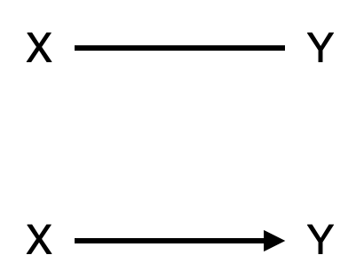
Many observational studies try to find a relationship between exposure and outcome. They typically report whether exposure and outcome are associated, and how. But as every student of statistics would know, correlation does not equal causation. What is meant by this is that if we find a correlation between an exposure and an outcome, this does not mean that the exposure causes the outcome. This is often framed as “correlation does not imply causation”, which is not entirely correct. In fact, correlation does imply causation somewhere - but the cause could be somewhere completely different. For example, the outcome could actually cause the exposure, or there could be other confounding factors that are responsible for linking the exposure to the outcome. Moreover, our data could already be heavily biased by the process through which it has been collected, generating the correlation. Thus, the correct statement would be “correlation between X and Y does not imply that X causes Y.”
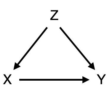
As an example, consider the causal diagram shown in Figure 3.10. We might be interested in understanding if the exposure X causes the outcome Y. Perhaps we have already established a strong association between the two. However, there could be a confounder X that influences both the exposure and the outcome. To use an often-mentioned example, consider the correlation between height (X) and mathematical ability (Y) in children. The taller the child, the higher the math competence. In this case, we intuitively understand that height doesn’t actually cause mathematical ability. Instead, age (Z) is a confounder, because age influences both height (through biological development) and mathematical ability (through schooling), explaining the observed correlation. In epidemiological studies, the situation is often not quite as straightforward as that. For example, we mentioned above that early case-control studies in the 1950ies showed that smoking and lung cancer are strongly associated. A subsequent prospective cohort study of British doctors confirmed the association. But this wasn’t enough to convince many people at the time. Some - including none other than R.A. Fisher, one of the founders of the statistical sciences - argued that the individual genotype could be a confounder, causing people to crave smoking as well as making them more susceptible to lung cancer6.
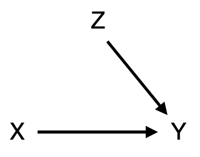
To his credit, Fisher is also the scientist to develop the ideal study design to establish causality, the randomized control trial. Fisher’s insight was that if we can assign the exposure X randomly, then we break any causal link between confounders and the exposure. In an RCT that is trying to establish a causal link between exposure X and outcome Y, our causal diagram would thus look like Figure 3.11. Through the random assignment of the exposure (e.g. a treatment), our exposed and non-exposed groups become comparable before we apply the exposure. Note that there can still be many factors Z affecting the outcome Y. But because of randomization, the effect of Z on the outcome Y is comparable in both groups, and any difference we observe in outcome Y is caused by exposure X.
Throughout most of the history of statistics, RCTs have been widely considered the only reliable means of establishing causality. Consequently, observational studies were thought to be entirely incapable of providing any insight into causation. If this were indeed the case, it would be highly problematic, because RCTs are often impossible for ethical or practical reasons. This is why you will (thankfully) never be reading about an RCT where participants were randomly assigned to start smoking. Today, we understand that while causality cannot be proven from observational models, we can nevertheless establish causality with some confidence, provided we are careful and explicit about the underlying causal model that generated our data. This is the domain of causal inference, which deals with the estimation of causal parameters in observational studies (Savitz and Wellenius 2022), and which has seen tremendous development and interest from the scientific community in the past 20 years. The mathematical framework behind causal inference is beyond the scope of this book, but readers are encouraged to explore the growing literature in this interesting area7.
Finally, even if we are not able to establish causation, associations can nonetheless be valuable. First, an association means that something interesting is going on somewhere, and we should find out where the association comes from. Secondly, an association, even if not causal, is valuable for prediction. A known association between X and Y allows us to predict Y if we know X, which can often be very useful. For example, many of the impressive results in artificial intelligence in recent years are the result of predictive power due to correlations learned from observational data. But in order to establish causality from observational data, we need to build causal models that incorporate expert knowledge (Robins 2001). We will now turn our attention to some key concepts that will help us build up our expert knowledge in the domain of infectious diseases.
https://vaccination-info.eu/en/vaccine-facts/approval-vaccines-european-union↩︎
https://onlinelibrary.wiley.com/doi/book/10.1002/9781119099369↩︎
https://onlinelibrary.wiley.com/doi/book/10.1002/9781119099369↩︎
https://community.cochrane.org/review-production/production-resources/living-systematic-reviews↩︎
A few interesting books: The Book of Why: The New Science of Cause and Effect, Causal Inference: What If, Causality: Models, Reasoning and Inference, Causal Inference in Statistics - A Primer, and Causal Inference: The Mixtape.↩︎